Reducing Probability to Arithmetic

Can we reduce aspects of probability and set theory to algebraic arithmetic? First, why would we even consider doing this?

Most of us spend years training our intuition and skills in arithmetic and algebraic manipulation, becoming quite proficient. When we then encounter the rules of set theory, Boolean logic, or probability, the operations often feel strangely familiar. Reminiscent of algebra, yet somehow distinct.

We might feel like we’re re-learning similar concepts in a different language. Probability, in particular, is known for its share of potentially confusing paradoxes and results that can defy initial intuition. Wouldn’t it be powerful if we could make the connection explicit? If we could merge these seemingly separate topics, we could leverage our strong foundation in algebra to build a more unified and perhaps more intuitive understanding. Let’s attempt to explore that connection today.

Sometimes in mathematics, you stumble upon a pattern that seems too structured to be a mere coincidence. It hints at a deeper connection, a different way of looking at things. Let’s explore one such instance, starting with a fundamental tool in probability: the Principle of Inclusion-Exclusion.

1. The Familiar Pattern of Inclusion-Exclusion

The Principle of Inclusion-Exclusion (PIE) gives us a way to calculate the probability that at least one of several events occurs – the probability of their union. For two events, it’s simple:

\[\Pr(A \cup B) = \Pr(A) + \Pr(B) - \Pr(A \cap B)\]

For three events, it expands:

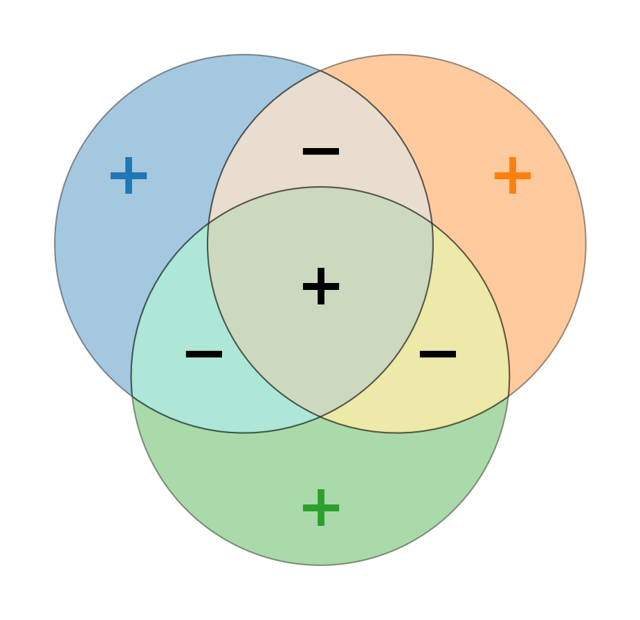
\[\begin{aligned} \Pr(A \cup B \cup C) &= [\Pr(A) + \Pr(B) + \Pr(C)] \\ &- [\Pr(A \cap B) + \Pr(A \cap C) + \Pr(B \cap C)] \\ &+ \Pr(A \cap B \cap C) \end{aligned}\]

The general formula for \(n\) events \(A_1, \dots, A_n\) involves summing probabilities of single events, subtracting probabilities of all pairwise intersections, adding probabilities of all triple intersections, and so on, with alternating signs. It is typically proven using induction and careful bookkeeping.

\[\begin{aligned} \Pr\left(\bigcup_{i=1}^n A_i\right) &= \sum_i \Pr(A_i) \\ &- \sum_{i<j} \Pr(A_i \cap A_j) \\ &+ \sum_{i<j<k} \Pr(A_i \cap A_j \cap A_k) \\ &- \dots \\ &+ (-1)^{n-1} \Pr(A_1 \cap \dots \cap A_n) \end{aligned}\]

Let’s define the sums of intersection probabilities:

• \[S_1 = \sum_i \Pr(A_i)\]
• \[S_2 = \sum_{i<j} \Pr(A_i \cap A_j)\]
• \[S_k = \sum_{1 \le i_1 < \dots < i_k \le n} \Pr(A_{i_1} \cap \dots \cap A_{i_k})\]

Then PIE can be written compactly as:

\[\Pr\left(\bigcup_{i=1}^n A_i\right) = S_1 - S_2 + S_3 - \dots + (-1)^{n-1} S_n\]

Now, consider the special symmetric case we discussed before: all single events have the same probability \(p_1\), all distinct pairs have the same intersection probability \(p_2\), etc., up to \(p_n\). The number of terms in \(S_k\) is \(\binom{n}{k}\), read \(n\) choose \(k\), defined as the number of ways to choose \(k\) items without order from \(n\) items. So, \(S_k = \binom{n}{k} p_k\). In this symmetric situation, the PIE formula becomes:

\[\Pr\left(\bigcup_{i=1}^n A_i\right) = \binom{n}{1} p_1 - \binom{n}{2} p_2 - \binom{n}{3} p_3 + \dots + (-1)^{n-1} \binom{n}{n} p_n\]

Crucially, this exact same pattern applies not just to probabilities, but also to calculating the size (cardinality) of the union of finite sets, where \(S_k\) would represent the sum of sizes of the intersection of any \(k\) sets. If \(\vert A_{i_1} \cap \dots \cap A_{i_k} \vert = s_k\) for any distinct \(i_1, \dots, i_k\), then \(\vert \cup A_i \vert = \binom{n}{1} s_1 - \binom{n}{2} s_2 + \dots\). The fact that this structure arises both in counting elements and in measuring probability suggests it reflects a fundamental property of how sets combine, one that seems intriguingly connected to algebra.

Take a moment to look at this structure again: \(S_1 - S_2 + S_3 - \dots\) or \(\binom{n}{1} p_1 - \binom{n}{2} p_2 + \dots\). The alternating signs and the summation over combinations (explicitly involving binomial coefficients in the symmetric case) feel deeply familiar to anyone who’s worked with algebraic expansions like:

\[(1-x)^n = \binom{n}{0} - \binom{n}{1} x + \binom{n}{2} x^2 - \binom{n}{3} x^3 + \dots + (-1)^n \binom{n}{n} x^n\]

Is this resemblance just superficial? Or does the Principle of Inclusion-Exclusion, applicable to both set sizes and probabilities, have an algebraic heart related to expansions like \((1-x)^n\)? This suspicion strongly motivates us to find a way to translate the language of set operations (\(\cup, \cap\)) into the language of algebra (\(+, -, \times\)).

2. Building a Bridge: Indicator Functions

How can we represent the occurrence or non-occurrence of an event numerically, in a way that algebraic operations naturally correspond to set operations? The answer lies in a wonderfully simple construction: the indicator function (also known as a characteristic function, but this terminology conflicts with statistics).

For any event \(A\) (which is just a subset of the sample space \(\Omega\)), its indicator function \(1_A\) is defined for each possible outcome \(\omega \in \Omega\):

\[1_A(\omega) = \begin{cases} 1 & \text{if } \omega \in A \\ 0 & \text{if } \omega \notin A \end{cases}\]

Think of it as a switch: it’s \(1\) (ON) if the outcome \(\omega\) makes the event \(A\) happen, and \(0\) (OFF) otherwise. The magic happens when we see how set operations translate into simple arithmetic:

• Intersection (\(\cap\)) becomes Multiplication (\(\times\)): An outcome \(\omega\) is in \(A \cap B\) if and only if it’s in both \(A\) and \(B\). This means \(1_{A \cap B}(\omega)\) should be \(1\) if and only if both \(1_A(\omega)\) and \(1_B(\omega)\) are \(1\). Simple multiplication achieves this perfectly because \(1 \times 1 = 1\), while \(1 \times 0 = 0\), \(0 \times 1 = 0\), and \(0 \times 0 = 0\).

  \[\boxed{1_{A \cap B} = 1_A \cdot 1_B}\]

  This extends to multiple events: \(1_{A_1 \cap \dots \cap A_n} = 1_{A_1} \cdot \dots \cdot 1_{A_n}\).

• Complement (\(^c\)) becomes Subtraction from 1: An outcome \(\omega\) is in \(A^c\) (the complement of \(A\)) if and only if it’s not in \(A\). So \(1_{A^c}(\omega)\) should be \(1\) when \(1_A(\omega)\) is \(0\), and vice versa.

  \[\boxed{1_{A^c} = 1 - 1_A}\]

These two rules are fundamental. We can derive others using them and basic set theory identities (like De Morgan’s laws):

• Union (\(\cup\)): Using \(A \cup B = (A^c \cap B^c)^c\), we get:

  \[1_{A \cup B} = 1 - 1_{(A \cup B)^c} = 1 - 1_{A^c \cap B^c} = 1 - (1_{A^c} \cdot 1_{B^c})\]

  Substituting \(1_{A^c} = 1 - 1_A\) and \(1_{B^c} = 1 - 1_B\):

  \[1_{A \cup B} = 1 - (1 - 1_A)(1 - 1_B) = 1 - (1 - 1_A - 1_B + 1_A 1_B)\] \[\boxed{1_{A \cup B} = 1_A + 1_B - 1_A 1_B = 1_A + 1_B - 1_{A \cap B}}\]

  Notice this already mirrors the PIE formula for two events!

• Set Difference (\(\setminus\)): Since \(A \setminus B = A \cap B^c\), we have:

  \[\boxed{1_{A \setminus B} = 1_A \cdot 1_{B^c} = 1_A (1 - 1_B) = 1_A - 1_A 1_B = 1_A - 1_{A \cap B}}\]

• Symmetric Difference (\(\Delta\)): \(A \Delta B = (A \setminus B) \cup (B \setminus A)\). Using the union formula on \(A \setminus B\) and \(B \setminus A\), which are disjoint:

  \[1_{A \Delta B} = 1_{A \setminus B} + 1_{B \setminus A} - 1_{(A \setminus B) \cap (B \setminus A)}\]

  Since the intersection is empty, its indicator is \(0\).

  \[1_{A \Delta B} = (1_A - 1_{A \cap B}) + (1_B - 1_{A \cap B}) = 1_A + 1_B - 2 \cdot 1_{A \cap B}\]

  Alternatively, using \(A \Delta B = (A \cup B) \setminus (A \cap B)\):

  \[1_{A \Delta B} = 1_{A \cup B} - 1_{(A \cup B) \cap (A \cap B)} = 1_{A \cup B} - 1_{A \cap B}\] \[1_{A \Delta B} = (1_A + 1_B - 1_{A \cap B}) - 1_{A \cap B} = 1_A + 1_B - 2 \cdot 1_{A \cap B}\]

  Also note that \(1_{A \Delta B}(\omega) = (1_A(\omega) - 1_B(\omega))^2\). This works because if both are \(0\) or both are \(1\), the difference is \(0\), squared is \(0\). If one is \(1\) and the other is \(0\), the difference is \(\pm 1\), squared is \(1\).

  \[\boxed{1_{A \Delta B} = (1_A - 1_B)^2 = 1_A + 1_B - 2 \cdot 1_{A \cap B}}\]

This translation is powerful. It allows us to rephrase statements about set relationships using algebraic equations involving these \(0/1\) functions. An interesting property is idempotence: \(1_A \cdot 1_A = 1_A\). This distinguishes this algebra from standard number algebra but is characteristic of Boolean algebra (where \(x \land x = x\)).

But we started with a question about probabilities. How do these indicator functions connect back to \(\Pr(A)\)?

3. Expectation: Linking Indicators to Probabilities

The connection is made through the concept of expectation, denoted \(\mathbb{E}[\cdot]\). The expectation of a random variable is its average value over the sample space, weighted by probabilities. For a simple random variable like an indicator function \(1_A\), which only takes values \(0\) or \(1\), the expectation is particularly straightforward:

\[\mathbb{E}[1_A] = \sum_{\omega \in \Omega} 1_A(\omega) \Pr(\omega)\]

We can split the sum based on whether \(\omega\) is in \(A\) or not:

\[\mathbb{E}[1_A] = \sum_{\omega \in A} 1 \cdot \Pr(\omega) + \sum_{\omega \notin A} 0 \cdot \Pr(\omega)\] \[\mathbb{E}[1_A] = \sum_{\omega \in A} \Pr(\omega) + 0\]

By the definition of the probability of an event, \(\Pr(A) = \sum_{\omega \in A} \Pr(\omega)\). Therefore:

\[\boxed{\mathbb{E}[1_A] = \Pr(A)}\]

This is the crucial link: The expectation of an indicator function is exactly the probability of the corresponding event.

Furthermore, expectation possesses a vital algebraic property: linearity. For any random variables \(X, Y\) (including indicator functions) and constants \(a, b\):

\[\mathbb{E}[aX + bY] = a\mathbb{E}[X] + b\mathbb{E}[Y]\]

This linearity holds regardless of whether \(X\) and \(Y\) are independent. It means we can perform algebraic manipulations on indicator functions (addition, subtraction, scalar multiplication) and then apply the expectation operator term by term to translate the result into a statement about probabilities.

4. Unveiling the Algebraic Root of PIE

Let’s revisit our goal: understanding the structure of \(\Pr(\cup A_i)\) using this algebraic framework. As before, it’s often easier to first consider the complement event: “none of the events \(A_i\) occur.” This corresponds to the intersection of the complements: \(\bigcap_{i=1}^n A_i^c\).

Using our indicator function toolkit:

• The indicator for the complement \(A_i^c\) is \(1_{A_i^c} = 1 - 1_{A_i}\).
• The indicator for the intersection \(\bigcap A_i^c\) is the product of the individual indicators: \(1_{\bigcap A_i^c} = \prod_{i=1}^n 1_{A_i^c} = \prod_{i=1}^n (1 - 1_{A_i})\)

Now, let’s expand this product algebraically, just like expanding \((1-x_1)(1-x_2)\dots(1-x_n)\) where we treat \(1_{A_i}\) as symbolic variables for a moment:

\[\prod_{i=1}^n (1 - 1_{A_i}) = 1 - \sum_i 1_{A_i} + \sum_{i<j} (1_{A_i} 1_{A_j}) - \sum_{i<j<k} (1_{A_i} 1_{A_j} 1_{A_k}) + \dots + (-1)^n (1_{A_1} \dots 1_{A_n})\]

Now, we use the crucial rule that the product of indicators corresponds to the indicator of the intersection: \(1_{A_i} 1_{A_j} = 1_{A_i \cap A_j}\), \(1_{A_i} 1_{A_j} 1_{A_k} = 1_{A_i \cap A_j \cap A_k}\), etc. Substituting these back:

\[1_{\bigcap A_i^c} = 1 - \sum_i 1_{A_i} + \sum_{i<j} 1_{A_i \cap A_j} - \sum_{i<j<k} 1_{A_i \cap A_j \cap A_k} + \dots + (-1)^n 1_{A_1 \cap \dots \cap A_n}\]

This equation is an identity holding true for any outcome \(\omega\). It relates the indicator of “none occur” to indicators of single events, intersections of pairs, triples, etc., with exactly the alternating signs we saw in PIE!

Now, let’s apply the expectation operator \(\mathbb{E}[\cdot]\) to both sides. Using its linearity and the fact that \(\mathbb{E}[1_E] = \Pr(E)\) for any event \(E\) (and \(\mathbb{E}[1] = 1\)):

\[\mathbb{E}[1_{\bigcap A_i^c}] = \mathbb{E}[1] - \sum_i \mathbb{E}[1_{A_i}] + \sum_{i<j} \mathbb{E}[1_{A_i \cap A_j}] - \dots + (-1)^n \mathbb{E}[1_{A_1 \cap \dots \cap A_n}]\] \[\Pr\left(\bigcap_{i=1}^n A_i^c\right) = 1 - \sum_i \Pr(A_i) + \sum_{i<j} \Pr(A_i \cap A_j) - \dots + (-1)^n \Pr(A_1 \cap \dots \cap A_n)\]

Using our \(S_k\) notation:

\[\Pr(\text{None occur}) = 1 - S_1 + S_2 - S_3 + \dots + (-1)^n S_n\]

Finally, the probability of the union (at least one event occurs) is 1 minus the probability that none occur:

\[\Pr\left(\bigcup_{i=1}^n A_i\right) = 1 - \Pr\left(\bigcap_{i=1}^n A_i^c\right)\]

Substituting the expression we just found:

\[\Pr\left(\bigcup_{i=1}^n A_i\right) = 1 - \left[ 1 - S_1 + S_2 - S_3 + \dots + (-1)^n S_n \right]\] \[\boxed{\Pr\left(\bigcup_{i=1}^n A_i\right) = S_1 - S_2 + S_3 - \dots + (-1)^{n-1} S_n}\]

We have recovered the Principle of Inclusion-Exclusion through purely algebraic manipulation of indicator functions followed by taking the expectation.

The key insight: The structure of PIE, with its alternating sums \(S_k\), directly mirrors the algebraic expansion of the product \(\prod (1 - 1_{A_i})\) when viewed through the lens of expectation. The binomial pattern we initially observed wasn’t a coincidence; it reflects an underlying algebraic identity made manifest through indicator functions.

5. Application: The Number of Events Occurring

Let’s push this algebraic approach further. Define a random variable \(N\) that counts how many of the events \(A_1, \dots, A_n\) occur for a given outcome \(\omega\). Using indicator functions, this is simply:

\[N = \sum_{i=1}^n 1_{A_i}\]

This elegantly represents the count: for any outcome \(\omega\), \(N(\omega)\) is the sum of 1s for the events that contain \(\omega\).

What is the expected number of events that occur? Using the linearity of expectation:

\[\mathbb{E}[N] = \mathbb{E}\left[\sum_{i=1}^n 1_{A_i}\right] = \sum_{i=1}^n \mathbb{E}[1_{A_i}] = \sum_{i=1}^n \Pr(A_i)\] \[\boxed{\mathbb{E}[N] = S_1}\]

This is intuitive: the average number of events occurring is simply the sum of their individual probabilities. This result is fundamental in many combinatorial arguments (like the probabilistic method).

Now, let’s calculate the variance of \(N\). Recall that \(\mathrm{Var}(N) = \mathbb{E}[N^2] - (\mathbb{E}[N])^2\). We already have \(\mathbb{E}[N] = S_1\). We need \(\mathbb{E}[N^2]\).

\[N^2 = \left(\sum_{i=1}^n 1_{A_i}\right) \left(\sum_{j=1}^n 1_{A_j}\right) = \sum_{i=1}^n \sum_{j=1}^n 1_{A_i} 1_{A_j}\]

We can split the sum into terms where \(i=j\) and terms where \(i \neq j\):

\[N^2 = \sum_{i=1}^n (1_{A_i} \cdot 1_{A_i}) + \sum_{i \neq j} (1_{A_i} 1_{A_j})\]

Using \(1_{A_i} \cdot 1_{A_i} = 1_{A_i}\) (idempotence) and \(1_{A_i} 1_{A_j} = 1_{A_i \cap A_j}\):

\[N^2 = \sum_{i=1}^n 1_{A_i} + \sum_{i \neq j} 1_{A_i \cap A_j}\]

Now, take the expectation:

\[\mathbb{E}[N^2] = \mathbb{E}\left[\sum_{i=1}^n 1_{A_i}\right] + \mathbb{E}\left[\sum_{i \neq j} 1_{A_i \cap A_j}\right]\] \[\mathbb{E}[N^2] = \sum_{i=1}^n \mathbb{E}[1_{A_i}] + \sum_{i \neq j} \mathbb{E}[1_{A_i \cap A_j}]\] \[\mathbb{E}[N^2] = \sum_{i=1}^n \Pr(A_i) + \sum_{i \neq j} \Pr(A_i \cap A_j)\]

Note that the second sum counts each pair \((i, j)\) with \(i \neq j\) once. This is equivalent to twice the sum over pairs where \(i < j\): \(\sum_{i \neq j} \Pr(A_i \cap A_j) = 2 \sum_{i<j} \Pr(A_i \cap A_j) = 2 S_2\). So,

\[\mathbb{E}[N^2] = S_1 + 2 S_2\]

Now we can find the variance:

\[\mathrm{Var}(N) = \mathbb{E}[N^2] - (\mathbb{E}[N])^2 = (S_1 + 2 S_2) - (S_1)^2\] \[\boxed{\mathrm{Var}(N) = \sum_i \Pr(A_i) + 2 \sum_{i<j} \Pr(A_i \cap A_j) - \left(\sum_i \Pr(A_i)\right)^2}\]

Alternatively, we can express this using covariances:

\[\mathrm{Var}(N) = \mathrm{Var}\left(\sum_i 1_{A_i}\right) = \sum_i \mathrm{Var}(1_{A_i}) + \sum_{i \neq j} \mathrm{Cov}(1_{A_i}, 1_{A_j})\]

Where:

• \[\mathrm{Var}(1_{A_i}) = \mathbb{E}[1_{A_i}^2] - (\mathbb{E}[1_{A_i}])^2 = \mathbb{E}[1_{A_i}] - (\mathbb{E}[1_{A_i}])^2 = \Pr(A_i) - \Pr(A_i)^2 = \Pr(A_i)(1-\Pr(A_i))\]
• \[\mathrm{Cov}(1_{A_i}, 1_{A_j}) = \mathbb{E}[1_{A_i} 1_{A_j}] - \mathbb{E}[1_{A_i}] \mathbb{E}[1_{A_j}] = \Pr(A_i \cap A_j) - \Pr(A_i)\Pr(A_j)\]

Substituting these in gives the same result, but highlights how variance depends on pairwise interactions (covariances/intersection probabilities relative to individual probabilities). This algebraic derivation using indicators is arguably much cleaner than combinatorial arguments.

6. Application: Probability of Exactly k Events

PIE gives the probability of at least one event (\(\Pr(N \ge 1)\)). We found \(\Pr(N=0)\) algebraically too. Can we find \(\Pr(N=k)\) for any \(k\)?

Let \(p_k = \Pr(N=k)\). We want to relate \(p_k\) to the sums \(S_j = \sum_{\vert I \vert=j} \Pr(\cap_{i \in I} A_i)\). There’s a known combinatorial identity:

\[p_k = \sum_{j=k}^n (-1)^{j-k} \binom{j}{k} S_j\]

Can we derive this using our algebraic approach? Let’s use generating functions. Consider the probability generating function (PGF) of \(N\):

\[P(x) = \mathbb{E}[x^N] = \sum_{k=0}^n \Pr(N=k) x^k = \sum_{k=0}^n p_k x^k\]

Now, let’s relate this to the sums \(S_j\). Consider the expectation of \(\binom{N}{j}\):

\[\binom{N}{j} = \binom{\sum_i 1_{A_i}}{j}\]

When we expand this binomial coefficient for a specific outcome \(\omega\), it counts the number of ways to choose \(j\) events from the set of events that actually occurred. Another way to think about this is:

\[\binom{N}{j}(\omega) = \sum_{1 \le i_1 < \dots < i_j \le n} 1_{A_{i_1}}(\omega) \dots 1_{A_{i_j}}(\omega) = \sum_{1 \le i_1 < \dots < i_j \le n} 1_{A_{i_1} \cap \dots \cap A_{i_j}}(\omega)\]

Taking the expectation:

\[\mathbb{E}\left[\binom{N}{j}\right] = \sum_{1 \le i_1 < \dots < i_j \le n} \mathbb{E}[1_{A_{i_1} \cap \dots \cap A_{i_j}}] = \sum_{1 \le i_1 < \dots < i_j \le n} \Pr(A_{i_1} \cap \dots \cap A_{i_j})\] \[\boxed{\mathbb{E}\left[\binom{N}{j}\right] = S_j}\]

The sums \(S_j\) are the binomial moments of the random variable \(N\).

Now, let’s connect the PGF \(P(x)\) to these binomial moments \(S_j\). Consider the expectation \(\mathbb{E}[(1+y)^N]\):

\[\mathbb{E}[(1+y)^N] = \mathbb{E}\left[\sum_{j=0}^N \binom{N}{j} y^j\right]\]

Assuming we can swap expectation and summation (which is fine for finite sums):

\[\mathbb{E}[(1+y)^N] = \sum_{j=0}^n \mathbb{E}\left[\binom{N}{j}\right] y^j = \sum_{j=0}^n S_j y^j\]

Let \(S(y) = \sum_{j=0}^n S_j y^j\) be the generating function for the binomial moments \(S_j\). We also know that \(P(x) = \mathbb{E}[x^N]\). If we substitute \(x = 1+y\), we get:

\[P(1+y) = \mathbb{E}[(1+y)^N] = S(y)\]

So, \(P(x) = S(x-1)\). Now we can substitute the series for \(S\):

\[P(x) = \sum_{j=0}^n S_j (x-1)^j\]

Expand \((x-1)^j\) using the binomial theorem: \((x-1)^j = \sum_{k=0}^j \binom{j}{k} x^k (-1)^{j-k}\).

\[P(x) = \sum_{j=0}^n S_j \left( \sum_{k=0}^j \binom{j}{k} x^k (-1)^{j-k} \right)\]

We want the coefficient of \(x^k\) in \(P(x)\), which is \(p_k\). We need to switch the order of summation. The term \(x^k\) appears when \(k \le j \le n\).

\[P(x) = \sum_{k=0}^n \left( \sum_{j=k}^n S_j \binom{j}{k} (-1)^{j-k} \right) x^k\]

By comparing the coefficients of \(x^k\) with \(P(x) = \sum_{k=0}^n p_k x^k\), we get:

\[\boxed{p_k = \Pr(N=k) = \sum_{j=k}^n (-1)^{j-k} \binom{j}{k} S_j}\]

This derivation beautifully showcases how algebraic manipulation of generating functions, linked via expectation and binomial moments (\(S_j\)), allows us to find the probability distribution of \(N\). It’s a powerful demonstration of reducing a potentially complex combinatorial probability problem to algebra.

7. Application: Bonferroni Inequalities

The PIE formula involves an alternating series: \(S_1 - S_2 + S_3 - \dots\). It’s known that for many alternating series where terms decrease in magnitude, the partial sums provide alternating bounds on the final sum. This holds true here and gives rise to the Bonferroni inequalities.

Recall the identity for the indicator of none occurring:

\[1_{\bigcap A_i^c} = 1 - \sum_i 1_{A_i} + \sum_{i<j} 1_{A_i \cap A_j} - \sum_{i<j<k} 1_{A_i \cap A_j \cap A_k} + \dots\]

Let \(T_k = \sum_{\vert I \vert=k} 1_{\cap_{i \in I} A_i}\). Then \(1_{\bigcap A_i^c} = 1 - T_1 + T_2 - T_3 + \dots\). It can be shown (though not trivially) that for any outcome \(\omega\):

• \[1 - T_1(\omega) \le 1_{\bigcap A_i^c}(\omega)\]
• \[1 - T_1(\omega) + T_2(\omega) \ge 1_{\bigcap A_i^c}(\omega)\]
• \(1 - T_1(\omega) + T_2(\omega) - T_3(\omega) \le 1_{\bigcap A_i^c}(\omega)\) And so on. Taking expectations maintains these inequalities:
• \(\mathbb{E}[1 - T_1] \le \mathbb{E}[1_{\bigcap A_i^c}]\) \(\implies 1 - S_1 \le \Pr(\text{None occur})\)
• \(\mathbb{E}[1 - T_1 + T_2] \ge \mathbb{E}[1_{\bigcap A_i^c}]\) \(\implies 1 - S_1 + S_2 \ge \Pr(\text{None occur})\)
• \[1 - S_1 + S_2 - S_3 \le \Pr(\text{None occur})\]

Since \(\Pr(\cup A_i) = 1 - \Pr(\text{None occur})\), we can flip the inequalities:

• From \(1 - S_1 \le 1 - \Pr(\cup A_i)\) \(\implies \Pr(\cup A_i) \le S_1\)
• From \(1 - S_1 + S_2 \ge 1 - \Pr(\cup A_i)\) \(\implies \Pr(\cup A_i) \ge S_1 - S_2\)
• From \(1 - S_1 + S_2 - S_3 \le 1 - \Pr(\cup A_i)\) \(\implies \Pr(\cup A_i) \le S_1 - S_2 + S_3\)

These are the Bonferroni inequalities: the partial sums of the PIE formula provide alternating upper and lower bounds on the true probability of the union. The algebraic structure of the underlying indicator identity \(1_{\cap A_i^c} = \sum (-1)^{\vert I \vert} 1_{\cap_{i \in I} A_i}\) is the foundation for these useful bounds.

8. Connection to Boolean Algebra

While we’ve focused on arithmetic (\(+, -, \times\)), it’s worth noting that indicator functions under different operations form a Boolean algebra. A common way to define Boolean operations is:

• AND (\(\land\)): \(1_A \land 1_B = \min(1_A, 1_B)\)
• OR (\(\lor\)): \(1_A \lor 1_B = \max(1_A, 1_B)\)
• NOT (\(\neg\)): \(\neg 1_A = 1 - 1_A\)

Notice the connections to our arithmetic operations:

• \(1_A \land 1_B = 1_A \cdot 1_B = 1_{A \cap B}\) (min behaves like product for \(0/1\) values)
• \(1_A \lor 1_B = 1_A + 1_B - 1_A 1_B = 1_{A \cup B}\) (max can be expressed arithmetically)
• \(\neg 1_A = 1_{A^c}\) (same as before)

This shows that the set of indicator functions on a sample space \(\Omega\), equipped with these operations, is algebraically identical (isomorphic) to the Boolean algebra of the subsets of \(\Omega\) (the events) equipped with (\(\cap, \cup, ^c\)). Our arithmetic approach (\(+, \times, 1-\)) provides an alternative, often more convenient, algebraic representation that directly links to expectation.

Conclusion: Seeing Probability Through Algebra

This journey started with a desire to connect the seemingly distinct rules of probability and set theory to the familiar world of algebra. We noticed a pattern in the Principle of Inclusion-Exclusion that echoed algebraic binomial expansions. By introducing indicator functions as a bridge (\(A \leftrightarrow 1_A\)) between set operations and arithmetic (\(\cap \leftrightarrow \times\), \(^c \leftrightarrow 1-\), \(\cup \leftrightarrow + - \times\)), and using the expectation operator (\(\mathbb{E}[1_A] = \Pr(A)\)) to link these back to probabilities, we uncovered the algebraic foundation of PIE. It arises naturally from expanding a product of terms like \((1 - 1_{A_i})\).

But the connection runs deeper. We saw how this algebraic perspective, centered on indicator functions and expectation, allows us to:

1. Derive PIE elegantly.
2. Calculate moments of the count variable \(N = \sum 1_{A_i}\), such as its expectation (\(\mathbb{E}[N]=S_1\)) and variance (\(\mathrm{Var}(N) = S_1 + 2S_2 - S_1^2\)).
3. Find the exact probability \(\Pr(N=k)\) using binomial moments (\(S_j = \mathbb{E}[\binom{N}{j}]\)) and generating functions.
4. Understand the origin of Bonferroni inequalities from the truncated algebraic expansion.
5. Relate directly to Boolean Algebra.

This algebraic viewpoint doesn’t replace the traditional set-theoretic or measure-theoretic foundations of probability, but it complements them beautifully. It provides a powerful computational tool, simplifies proofs, reveals hidden structures (like the role of binomial moments), and offers a different kind of intuition grounded in familiar algebraic manipulations. Recognizing these connections allows us to wield the tools of algebra to better understand and solve problems in probability and combinatorics, showing that sometimes, looking at a familiar concept from a different algebraic angle can reveal surprising elegance and utility.