Linear Algebra Part 1: Foundations & Geometric Transformations
A crash course on the foundational concepts of linear algebra from a geometric perspective, covering vectors, vector spaces, linear transformations, matrices, determinants, and systems of linear equations.
Linear algebra is the backbone of countless scientific and engineering disciplines. This first part of our crash course explores linear algebra from a geometric viewpoint, focusing on the foundational concepts in Euclidean spaces (\(\mathbb{R}^2\) and \(\mathbb{R}^3\)) where we can visualize them. We’ll cover vectors, vector spaces, linear transformations, matrices, determinants, and how these concepts relate to solving systems of linear equations.
There are great resources and visualizations done by others. For instance, I highly recommend Gregory Gunderson’s blog or Grant Sanderson’s (aka 3Blue1Brown) work both on YouTube and Khan Academy. Also, Fields medalist James Maynard’s Oxford lectures on Linear Algebra II is incredibly insightful, really building the intuition from scratch geometrically without assuming proven theorems as obvious or axiomatic as is typical of textbooks on the topic. These inspired the general approach of this post and many of the ideas presented here.
1. The Stage: Vectors and Vector Spaces
Our discussion begins with the fundamental objects of linear algebra: vectors.
Definition. Vector
Geometrically, a vector in \(\mathbb{R}^n\) is an arrow originating from a central point (the origin \(\vec{0}\)) and pointing to a coordinate \((x_1, x_2, \dots, x_n)\). It encapsulates both direction and magnitude (length). For example, \(\vec{v} = \begin{pmatrix} 2 \\ 1 \end{pmatrix}\) in \(\mathbb{R}^2\) is an arrow from \((0,0)\) to \((2,1)\). Vectors are often written as column matrices.
As we will see, this is the most naive definition of vectors that is typically used in a first presentation. We’ll start by working with it to build intuition, but we’ll eventually bring it to higher abstraction levels in order to make them more general and powerful.
Vector \(\begin{pmatrix} 2 \\ 1 \end{pmatrix}\) in \(\mathbb{R}^2\)
Vectors can be manipulated through two primary operations:
- Vector Addition: \(\vec{u} + \vec{v}\). Geometrically, place the tail of vector \(\vec{v}\) at the head (tip) of vector \(\vec{u}\). The sum \(\vec{u} + \vec{v}\) is the new vector from the origin (or tail of \(\vec{u}\)) to the head of the translated \(\vec{v}\). This is sometimes called the parallelogram law, as \(\vec{u}\), \(\vec{v}\), and \(\vec{u}+\vec{v}\) form three sides of a parallelogram if they share the same origin. However, the parallelogram law in more advanced contexts also refers to a different theorem relating the sides and the diagonals of a parallelogram, so you can also call it “tip to tail” vector addition, since at the tip of the first vector, you place the tail of the second.
- Scalar Multiplication: \(c\vec{v}\), where \(c\) is a scalar (a real number, unless stated otherwise). This operation scales the vector \(\vec{v}\).
- If \(\vert c \vert > 1\), the vector is stretched.
- If \(0 < \vert c \vert < 1\), the vector is shrunk.
- If \(c > 0\), the direction remains the same.
- If \(c < 0\), the direction is reversed.
- If \(c = 0\), the result is the zero vector \(\vec{0}\) (a point at the origin).
A vector space is a collection of vectors where these operations (addition and scalar multiplication) are well-defined and follow a set of axioms (associativity, commutativity, distributivity, existence of a zero vector, additive inverses, etc.). For our purposes, \(\mathbb{R}^n\) with the standard vector addition and scalar multiplication is the quintessential vector space. The formal definition of an abstract vector space will be discussed in Part 2 of this linear algebra series.
Example. Vector Operations
Let \(\vec{u} = \begin{pmatrix} 1 \\ 2 \end{pmatrix}\) and \(\vec{v} = \begin{pmatrix} 3 \\ -1 \end{pmatrix}\).
Sum:
\[\vec{u} + \vec{v} = \begin{pmatrix} 1 \\ 2 \end{pmatrix} + \begin{pmatrix} 3 \\ -1 \end{pmatrix} = \begin{pmatrix} 1+3 \\ 2+(-1) \end{pmatrix} = \begin{pmatrix} 4 \\ 1 \end{pmatrix}\]Geometrically, start at the origin, move to \((1,2)\), then from \((1,2)\) move 3 units right and 1 unit down. You end up at \((4,1)\).
Scalar Multiple:
\[2\vec{u} = 2 \begin{pmatrix} 1 \\ 2 \end{pmatrix} = \begin{pmatrix} 2 \cdot 1 \\ 2 \cdot 2 \end{pmatrix} = \begin{pmatrix} 2 \\ 4 \end{pmatrix}\]This vector points in the same direction as \(\vec{u}\) but is twice as long.
\[- \vec{v} = -1 \begin{pmatrix} 3 \\ -1 \end{pmatrix} = \begin{pmatrix} -3 \\ 1 \end{pmatrix}\]This vector has the same length as \(\vec{v}\) but points in the opposite direction.
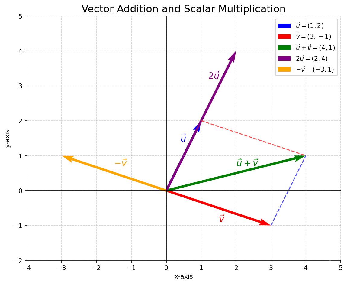 Example: Vector addition and scalar multiplication
1.1. Measuring Within Space: Dot Product, Length, and Orthogonality
The dot product (or standard inner product) introduces geometric notions of length and angle into \(\mathbb{R}^n\).
Definition. Dot Product
For two vectors \(\vec{u} = \begin{pmatrix} u_1 \\ \vdots \\ u_n \end{pmatrix}\) and \(\vec{v} = \begin{pmatrix} v_1 \\ \vdots \\ v_n \end{pmatrix}\) in \(\mathbb{R}^n\), their dot product is:
\[\vec{u} \cdot \vec{v} = u_1v_1 + u_2v_2 + \dots + u_nv_n = \sum_{i=1}^n u_i v_i\]Note: \(\vec{u} \cdot \vec{v} = \vec{u}^T \vec{v}\) if vectors are columns. Geometrically, the dot product is also defined as:
\[\vec{u} \cdot \vec{v} = \Vert \vec{u} \Vert \ \Vert \vec{v} \Vert \cos \theta\]where \(\Vert \vec{u} \Vert\) and \(\Vert \vec{v} \Vert\) are the magnitudes (lengths) of the vectors, \(\theta\) is the angle between them, and \(\Vert \cdot \Vert := \Vert \cdot \Vert_2\) denotes the Euclidean norm (length) of a vector. Note that the dot product in \(\mathbb{R}^n\) is a specific case of an inner product, because it gives the component of one vector that lies “inside” (in the direction of) the other by orthogonal projection.
\[\mathrm{proj}_\vec{u} \vec{v}=(\Vert \vec{v} \Vert \cos \theta) \frac{\vec{u}}{\Vert \vec{u} \Vert}\]Thus
\[\vert \vec{u} \cdot \vec{v} \vert = \Vert \vec{u} \Vert \Vert \mathrm{proj}_\vec{u} \vec{v} \Vert = \Vert \vec{u} \Vert \Vert \mathrm{proj}_\vec{v} \vec{u} \Vert\]and the sign is determined by \(\cos\theta\):
\[\begin{cases} \theta \in [0, \pi/2) & \Rightarrow \vec{u} \cdot \vec{v} \gt 0 \\ \theta = \pi/2 & \Rightarrow \vec{u} \cdot \vec{v} = 0 \\ \theta \in (\pi/2, \pi] & \Rightarrow \vec{u} \cdot \vec{v} \lt 0 \end{cases}\]In words, an acute angle between two vectors means they are positively correlated, an obtuse angle means they are negatively correlated, and a right angle means they are uncorrelated (orthogonal).
Dot product and angles
See (Gregory Gunderson, 2018) for in-depth explanation and geometric visualization.
Details. Derivation: Equivalence of Geometric and Algebraic Dot Product (2D)
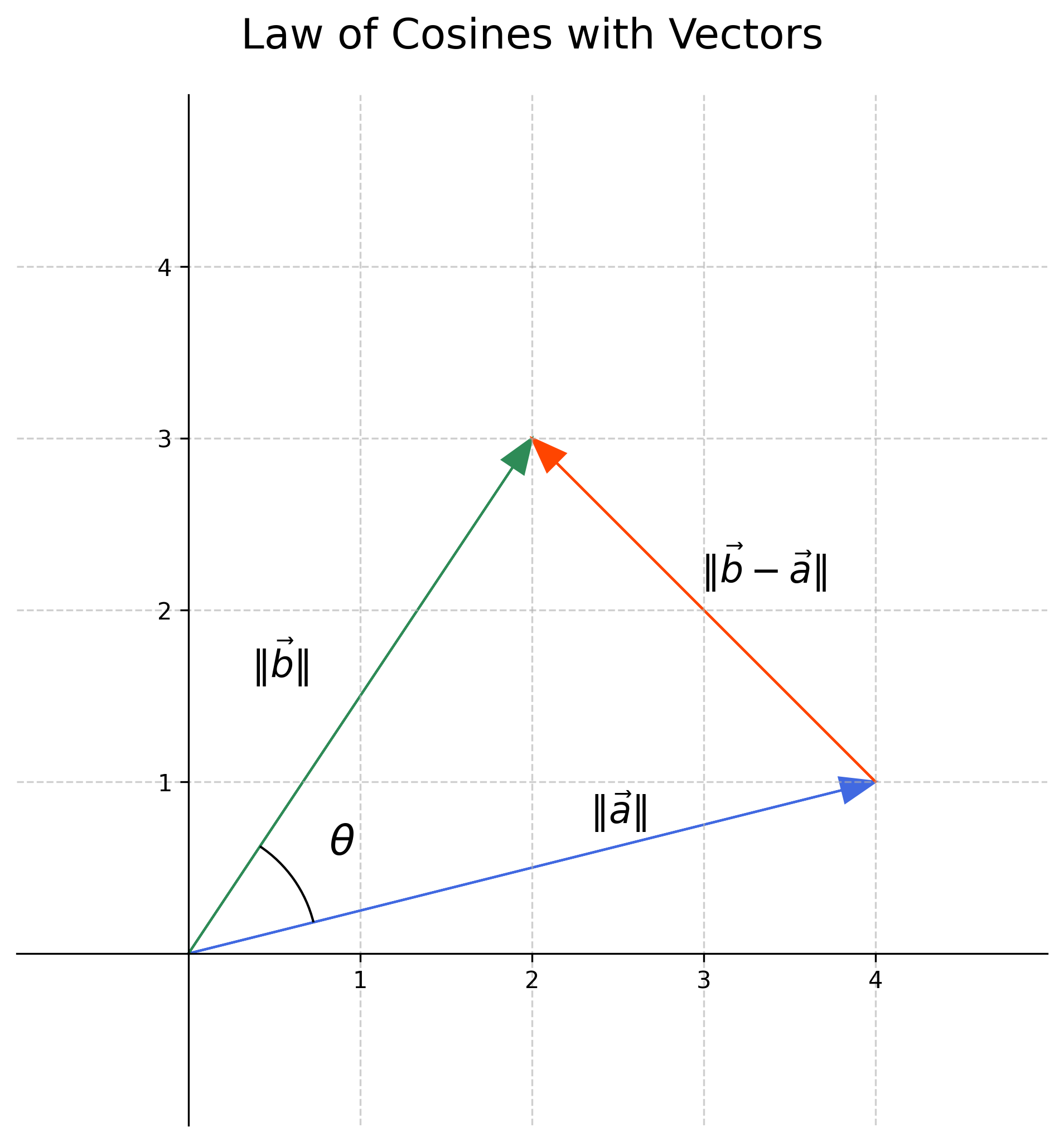
Consider two vectors \(\vec{a} = \begin{pmatrix} a_1 \\ a_2 \end{pmatrix}\) and \(\vec{b} = \begin{pmatrix} b_1 \\ b_2 \end{pmatrix}\). Let \(\theta\) be the angle between them. By the Law of Cosines on the triangle formed by \(\vec{a}\), \(\vec{b}\), and \(\vec{b}-\vec{a}\):
\[\Vert \vec{b}-\vec{a} \Vert ^2 = \Vert \vec{a} \Vert ^2 + \Vert \vec{b} \Vert ^2 - 2 \Vert \vec{a} \Vert \Vert \vec{b} \Vert \cos\theta\]We know \(\Vert \vec{a} \Vert \Vert \vec{b} \Vert \cos\theta\) is the geometric dot product, so let’s call it \((\vec{a} \cdot \vec{b})_{\text{geom}}\).
\[2 (\vec{a} \cdot \vec{b})_{\text{geom}} = \Vert \vec{a} \Vert ^2 + \Vert \vec{b} \Vert ^2 - \Vert \vec{b}-\vec{a} \Vert ^2\]Let’s expand the terms using coordinates:
\(\Vert \vec{a} \Vert ^2 = a_1^2 + a_2^2\) \(\Vert \vec{b} \Vert ^2 = b_1^2 + b_2^2\) \(\vec{b}-\vec{a} = \begin{pmatrix} b_1-a_1 \\ b_2-a_2 \end{pmatrix}\)
\[\Vert \vec{b}-\vec{a} \Vert ^2 = (b_1-a_1)^2 + (b_2-a_2)^2 = b_1^2 - 2a_1b_1 + a_1^2 + b_2^2 - 2a_2b_2 + a_2^2\]Substituting these into the equation for \(2 (\vec{a} \cdot \vec{b})_{\text{geom}}\):
\[2 (\vec{a} \cdot \vec{b})_{\text{geom}} = (a_1^2 + a_2^2) + (b_1^2 + b_2^2) - (b_1^2 - 2a_1b_1 + a_1^2 + b_2^2 - 2a_2b_2 + a_2^2)\] \[2 (\vec{a} \cdot \vec{b})_{\text{geom}} = a_1^2 + a_2^2 + b_1^2 + b_2^2 - b_1^2 + 2a_1b_1 - a_1^2 - b_2^2 + 2a_2b_2 - a_2^2\]Many terms cancel out:
\[2 (\vec{a} \cdot \vec{b})_{\text{geom}} = 2a_1b_1 + 2a_2b_2\] \[(\vec{a} \cdot \vec{b})_{\text{geom}} = a_1b_1 + a_2b_2\]This is precisely the algebraic definition of the dot product. The derivation extends to higher dimensions.
The dot product connects to geometry through:
Length (Norm): The length of a vector \(\vec{v}\) is
\[\Vert \vec{v} \Vert = \sqrt{\vec{v} \cdot \vec{v}} = \sqrt{v_1^2 + v_2^2 + \dots + v_n^2}\]Angle: The angle \(\theta\) between two non-zero vectors \(\vec{u}\) and \(\vec{v}\) is given by:
\[\cos \theta = \frac{\vec{u} \cdot \vec{v}}{ \Vert \vec{u} \Vert \ \Vert \vec{v} \Vert }\]Orthogonality: Two vectors \(\vec{u}\) and \(\vec{v}\) are orthogonal (perpendicular) if their dot product is zero:
\[\vec{u} \cdot \vec{v} = 0\](This is because if \(\theta = 90^\circ\), then \(\cos \theta = 0\)). Orthogonality is a central theme that will be explored further in Part 2.
Example. Dot Product and Angle
Let \(\vec{u} = \begin{pmatrix} 1 \\ 1 \end{pmatrix}\) and \(\vec{v} = \begin{pmatrix} 1 \\ 0 \end{pmatrix}\).
- \[\vec{u} \cdot \vec{v} = (1)(1) + (1)(0) = 1\]
- \[\Vert \vec{u} \Vert = \sqrt{1^2+1^2} = \sqrt{2}\]
- \[\Vert \vec{v} \Vert = \sqrt{1^2+0^2} = \sqrt{1} = 1\]
- Angle \(\theta\): \(\cos \theta = \frac{1}{\sqrt{2} \cdot 1} = \frac{1}{\sqrt{2}}\). So \(\theta = 45^\circ\) or \(\pi/4\) radians. This makes sense geometrically: \(\vec{u}\) points along the line \(y=x\), and \(\vec{v}\) points along the x-axis.
Vector Projection: The projection of vector \(\vec{u}\) onto vector \(\vec{v}\) (the “shadow” of \(\vec{u}\) on the line defined by \(\vec{v}\)) is:
\[\text{proj}_{\vec{v}} \vec{u} = \underbrace{\vec{u}\cdot \left(\frac{\vec{v}}{\Vert \vec{v} \Vert} \right)}_{\text{signed length}} \underbrace{\frac{\vec{v}}{\Vert \vec{v} \Vert}}_{\text{direction}} = \frac{\vec{u} \cdot \vec{v}}{ \Vert \vec{v} \Vert ^2} \vec{v}\]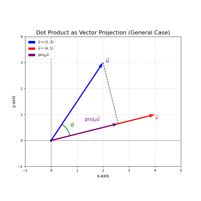 Vector projection
The scalar part \(\frac{\vec{u} \cdot \vec{v}}{ \Vert \vec{v} \Vert }\) is the signed length of this projection. Projections onto subspaces will be covered in Part 2.
1.2. The Cross Product (for \(\mathbb{R}^3\)): Orthogonal Vectors and Area
The cross product is an operation between two vectors in 3D space that results in another 3D vector.
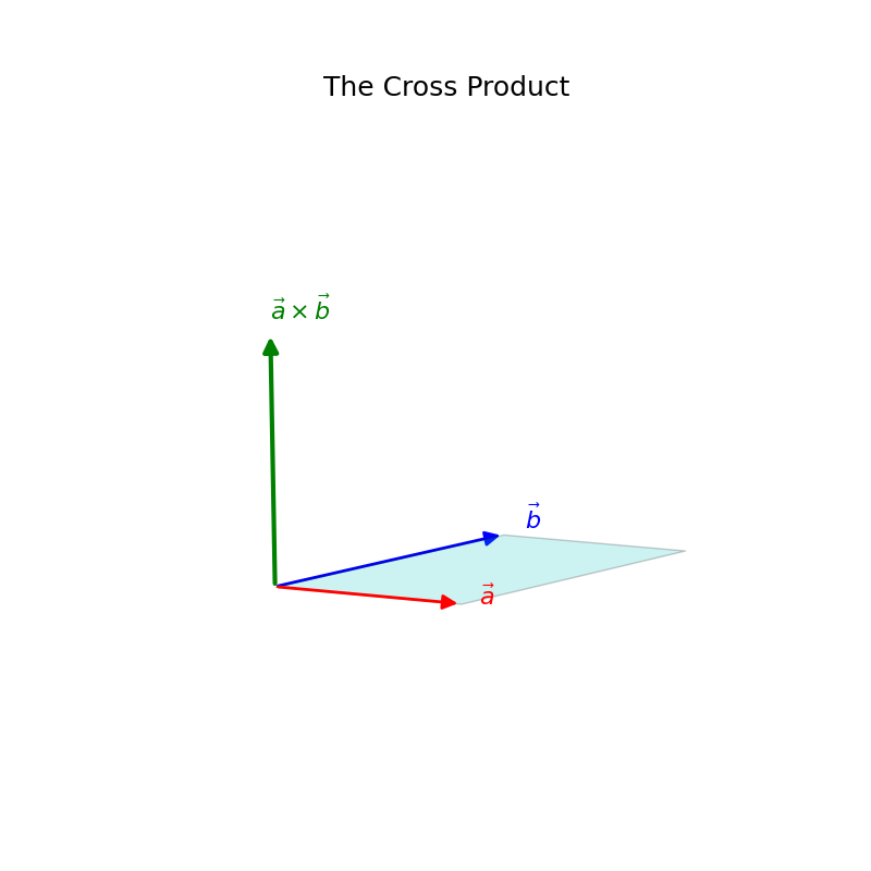
Definition. Cross Product
The cross product of two vectors \(\vec{a}\) and \(\vec{b}\) in \(\mathbb{R}^3\), denoted \(\vec{a} \times \vec{b}\), is a vector \(\vec{c}\) such that:
- Direction: \(\vec{c}\) is orthogonal (perpendicular) to both \(\vec{a}\) and \(\vec{b}\). Its specific direction is given by the right-hand rule (point fingers of right hand along \(\vec{a}\), curl towards \(\vec{b}\), thumb points in direction of \(\vec{a} \times \vec{b}\)).
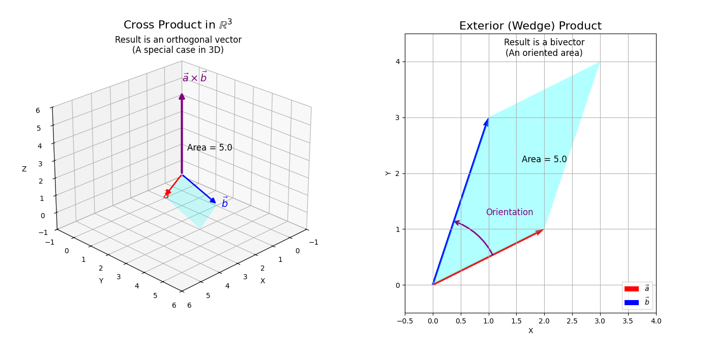
- Magnitude: \(\Vert \vec{a} \times \vec{b} \Vert = \Vert \vec{a} \Vert \Vert \vec{b} \Vert \sin\theta\), where \(\theta\) is the angle between \(\vec{a}\) and \(\vec{b}\). This magnitude is equal to the area of the parallelogram spanned by \(\vec{a}\) and \(\vec{b}\).
Algebraically, if \(\vec{a} = \begin{pmatrix} a_1 \\ a_2 \\ a_3 \end{pmatrix}\) and \(\vec{b} = \begin{pmatrix} b_1 \\ b_2 \\ b_3 \end{pmatrix}\):
\[\vec{a} \times \vec{b} = \begin{pmatrix} a_2 b_3 - a_3 b_2 \\ a_3 b_1 - a_1 b_3 \\ a_1 b_2 - a_2 b_1 \end{pmatrix}\]Note that \(\vec{a} \times \vec{b} = - (\vec{b} \times \vec{a})\) (it’s anti-commutative). Also, if \(\vec{a}\) and \(\vec{b}\) are parallel or anti-parallel (\(\theta=0^\circ\) or \(\theta=180^\circ\)), then \(\sin\theta=0\), so \(\vec{a} \times \vec{b} = \vec{0}\).
Details. The Wedge Product, A More Natural Cross Product
The cross product is actually a pretty unnatural concept. If you have used it in engineering contexts, you know that it’s often used to represent quantities about rotation, e.g. torque. However, this is very unnatural. A rotation happens in a plane, i.e. a 2D subspace. So why do we need to introduce an additional third dimension to solve problems? The answer is that we shouldn’t. We can work directly in that plane.
You have likely heard the statement that “you can’t multiply two vectors like you multiply two scalars”. Supposedly, you can only use the dot product OR the cross product. If you’ve ever played with complex numbers, though, you might have found some curious behavior that makes the following exploration less surprising. A complex number is essentially like a 2D vector, having two perpendicular coordinates:
\[a+ib\cong \begin{pmatrix} a \\ b \end{pmatrix}\]where \(i^2 = -1\). We also know that multiplication of complex numbers is well-defined:
\[(a+ib)(c+id)=(ac-bd)+i(ad+bc)\]Yet, we are supposed to believe that we can multiply complex numbers, but not 2D vectors? Of course, that doesn’t make sense. Look at the following:
\[\overline{(a+ib)}(c+id)=(a-ib)(c+id)=(ac+bd)+i(ad-bc)\]What do you notice about the real part of this product? Indeed, it’s precisely the dot product!
\[\begin{pmatrix} a \\ b \end{pmatrix} \cdot \begin{pmatrix} c \\ d \end{pmatrix} = ac+bd\]And if you already have seen some linear algebra before, you’ll be even more suspicious, as the imaginary part is precisely the determinant.
\[\begin{vmatrix} a & c \\ b & d \end{vmatrix} = ad-bc\]This provides motivation for a more general product between two vectors that is very similar.
The cross product as defined for \(\mathbb{R}^3\) is a special case of a more fundamental concept from exterior algebra: the exterior product (or wedge product), denoted \(\vec{u} \wedge \vec{v}\). In geometric algebra, we define the product between two vectors as:
\[\vec{a}\vec{b}=\vec{a} \cdot \vec{b}+\vec{a} \wedge \vec{b}.\]While the inner product (dot product) \(\vec{u} \cdot \vec{v}\) takes two vectors and produces a scalar (capturing notions of projection and angle), the exterior product \(\vec{u} \wedge \vec{v}\) takes two vectors and produces a different kind of algebraic object called a bivector.
Just like our vectors are “oriented line segments”, we can think of bivectors as an “oriented plane segment”.
- Geometric Meaning: A bivector \(\vec{u} \wedge \vec{v}\) represents an oriented parallelogram (an area element) in the plane spanned by \(\vec{u}\) and \(\vec{v}\). Its magnitude is the area of this parallelogram, and its orientation indicates the sense of circulation from \(\vec{u}\) to \(\vec{v}\).
- Connection to Cross Product (in \(\mathbb{R}^3\)): In the specific case of \(\mathbb{R}^3\), there’s a unique correspondence (via the Hodge dual) between bivectors and vectors. The bivector \(\vec{u} \wedge \vec{v}\) can be associated with a vector that is orthogonal to the plane of \(\vec{u}\) and \(\vec{v}\), and whose magnitude is the area of the parallelogram they span. This associated vector is precisely the cross product \(\vec{u} \times \vec{v}\). In other dimensions (e.g., \(\mathbb{R}^2\) or \(\mathbb{R}^4\)), the wedge product of two vectors doesn’t naturally yield another vector in the same space in this way. For instance, in \(\mathbb{R}^2\), \(\vec{e}_1 \wedge \vec{e}_2\) is a bivector representing the unit area, akin to a scalar for orientation purposes.
- Why not in basic Linear Algebra? While the exterior product is itself bilinear (e.g., \((c\vec{u}) \wedge \vec{v} = c(\vec{u} \wedge \vec{v})\)), incorporating such products between vectors systematically leads to richer algebraic structures known as exterior algebras (or Grassmann algebras). These are the domain of multilinear algebra and tensor algebra. A standard linear algebra course primarily focuses on vector spaces and linear transformations mapping vectors to vectors, rather than products of vectors that yield new types of algebraic objects.
So, while the cross product is a very useful tool in 3D geometry and physics, its “true nature” as a part of exterior algebra is a more advanced topic.
Details. Pseudovectors: The “Weirdness” of Cross Product under Reflection
The fact that the cross product in \(\mathbb{R}^3\) is a pseudovector (or axial vector) rather than a true vector (or polar vector) leads to some counter-intuitive behaviors under transformations that change the “handedness” of the coordinate system, like reflections.
Imagine you have two vectors \(\vec{u}\) and \(\vec{v}\), and their cross product \(\vec{w} = \vec{u} \times \vec{v}\). Its direction is given by the right-hand rule.
Now, consider reflecting this entire scenario in a mirror:
- The vectors \(\vec{u}\) and \(\vec{v}\) are reflected to their mirror images, \(\vec{u}'\) and \(\vec{v}'\).
- If \(\vec{w}\) were a true (polar) vector, its mirror image, let’s call it \(\vec{w}_{\text{reflected arrow}}\), would simply be the geometric reflection of the arrow \(\vec{w}\).
- However, if you recalculate the cross product using the reflected input vectors, \(\vec{w}_{\text{recalculated}} = \vec{u}' \times \vec{v}'\) (using the same right-hand rule definition but now applied to the mirrored input vectors), you’ll find that \(\vec{w}_{\text{recalculated}} = -\vec{w}_{\text{reflected arrow}}\) for reflections that invert handedness.
Example: Let \(\vec{u} = \vec{e}_1 = \begin{pmatrix} 1 \\ 0 \\ 0 \end{pmatrix}\) and \(\vec{v} = \vec{e}_2 = \begin{pmatrix} 0 \\ 1 \\ 0 \end{pmatrix}\). Then their cross product is \(\vec{w} = \vec{u} \times \vec{v} = \vec{e}_3 = \begin{pmatrix} 0 \\ 0 \\ 1 \end{pmatrix}\).
Consider a reflection across the x-y plane. This transformation maps a point \((x,y,z)\) to \((x,y,-z)\).
- The reflection of \(\vec{u}\) is \(\vec{u}' = \begin{pmatrix} 1 \\ 0 \\ 0 \end{pmatrix}\) (it’s in the x-y plane, so it’s unchanged).
- The reflection of \(\vec{v}\) is \(\vec{v}' = \begin{pmatrix} 0 \\ 1 \\ 0 \end{pmatrix}\) (also unchanged).
- The cross product recalculated from these reflected vectors is \(\vec{w}_{\text{recalculated}} = \vec{u}' \times \vec{v}' = \begin{pmatrix} 1 \\ 0 \\ 0 \end{pmatrix} \times \begin{pmatrix} 0 \\ 1 \\ 0 \end{pmatrix} = \begin{pmatrix} 0 \\ 0 \\ 1 \end{pmatrix}\).
- However, the geometric reflection of the original \(\vec{w} = \begin{pmatrix} 0 \\ 0 \\ 1 \end{pmatrix}\) across the x-y plane is \(\vec{w}_{\text{reflected arrow}} = \begin{pmatrix} 0 \\ 0 \\ -1 \end{pmatrix}\).
Notice that \(\vec{w}_{\text{recalculated}} = (0,0,1)\) while \(\vec{w}_{\text{reflected arrow}} = (0,0,-1)\). They differ by a sign.
Intuition via the Right-Hand Rule and a Mirror:
- Hold up your right hand: your thumb points in the direction of \(\vec{w} = \vec{u} \times \vec{v}\) when your fingers curl from \(\vec{u}\) to \(\vec{v}\).
- Look at your right hand in a mirror.
- Your physical thumb has a mirror image. This direction corresponds to \(\vec{w}_{\text{reflected arrow}}\).
- The way your fingers appear to curl in the mirror (from mirror image \(\vec{u}'\) to mirror image \(\vec{v}'\)) is reversed. If your real fingers curl counter-clockwise (viewed from your eyes down your arm), the mirrored fingers appear to curl clockwise (viewed from the mirror image eyes down the mirror image arm).
- If you were to apply the right-hand rule to this apparent mirrored curl (clockwise), the thumb of this “rule-applying hand” would point in the direction opposite to \(\vec{w}_{\text{reflected arrow}}\). This new direction is \(\vec{w}_{\text{recalculated}}\).
This discrepancy (\(\vec{w}_{\text{recalculated}} = -\vec{w}_{\text{reflected arrow}}\)) is characteristic of pseudovectors. Quantities like angular velocity, torque, and magnetic field are pseudovectors. The bivector \(\vec{u} \wedge \vec{v}\), representing the oriented plane area, transforms more naturally under such operations. The issue arises because its common representation as a vector in \(\mathbb{R}^3\) (the cross product) is tied to the right-hand rule convention, which is sensitive to the coordinate system’s orientation or “handedness.”
Example. Cross product.
Let \(\vec{e}_1 = \begin{pmatrix} 1 \\ 0 \\ 0 \end{pmatrix}\) and \(\vec{e}_2 = \begin{pmatrix} 0 \\ 1 \\ 0 \end{pmatrix}\).
\[\vec{e}_1 \times \vec{e}_2 = \begin{pmatrix} (0)(0) - (0)(1) \\ (0)(0) - (1)(0) \\ (1)(1) - (0)(0) \end{pmatrix} = \begin{pmatrix} 0 \\ 0 \\ 1 \end{pmatrix} = \vec{e}_3\]Geometrically: \(\vec{e}_1\) and \(\vec{e}_2\) are orthogonal (\(\theta=90^\circ, \sin\theta=1\)), their lengths are 1. The area of the unit square they form is 1. The vector \(\vec{e}_3\) is orthogonal to both and follows the right-hand rule.
Vector Operations Exercises:
- Let \(\vec{a} = \begin{pmatrix} -2 \\ 3 \end{pmatrix}\) and \(\vec{b} = \begin{pmatrix} 4 \\ 1 \end{pmatrix}\). Calculate and draw \(\vec{a} + \vec{b}\), \(\vec{a} - \vec{b}\), and \(3\vec{a}\).
- Given \(\vec{u} = \begin{pmatrix} -1 \\ 2 \\ 3 \end{pmatrix}\) and \(\vec{v} = \begin{pmatrix} 4 \\ 0 \\ -2 \end{pmatrix}\). Calculate: a. \(\vec{u} + \vec{v}\) b. \(3\vec{u} - \frac{1}{2}\vec{v}\) c. \(\Vert \vec{u} \Vert\) d. \(\vec{u} \cdot \vec{v}\) e. The angle \(\theta\) between \(\vec{u}\) and \(\vec{v}\).
- Find a unit vector (length 1) in the direction of \(\vec{w} = \begin{pmatrix} 3 \\ -4 \\ 0 \end{pmatrix}\).
- For \(\vec{p} = \begin{pmatrix} 1 \\ 1 \\ 0 \end{pmatrix}\) and \(\vec{q} = \begin{pmatrix} 0 \\ 1 \\ 1 \end{pmatrix}\), calculate \(\vec{p} \times \vec{q}\). Verify that the resulting vector is orthogonal to both \(\vec{p}\) and \(\vec{q}\) using the dot product.
- Find the projection of \(\vec{u} = \begin{pmatrix} 2 \\ 3 \\ 1 \end{pmatrix}\) onto \(\vec{v} = \begin{pmatrix} 1 \\ 0 \\ -1 \end{pmatrix}\).
2. Building Blocks: Span, Linear Independence, Basis, Dimension
These concepts help us understand the structure within vector spaces.
Definition. Linear Combination
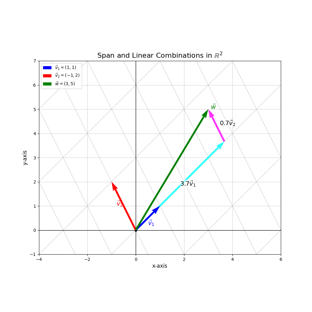
A linear combination of a set of vectors \(\{\vec{v}_1, \vec{v}_2, \dots, \vec{v}_k\}\) is any vector of the form:
\[\vec{w} = c_1\vec{v}_1 + c_2\vec{v}_2 + \dots + c_k\vec{v}_k\]where \(c_1, c_2, \dots, c_k\) are scalars. Geometrically, it’s the vector reached by stretching/shrinking/flipping the vectors \(\vec{v}_i\) and then adding them head-to-tail.
Definition. Span
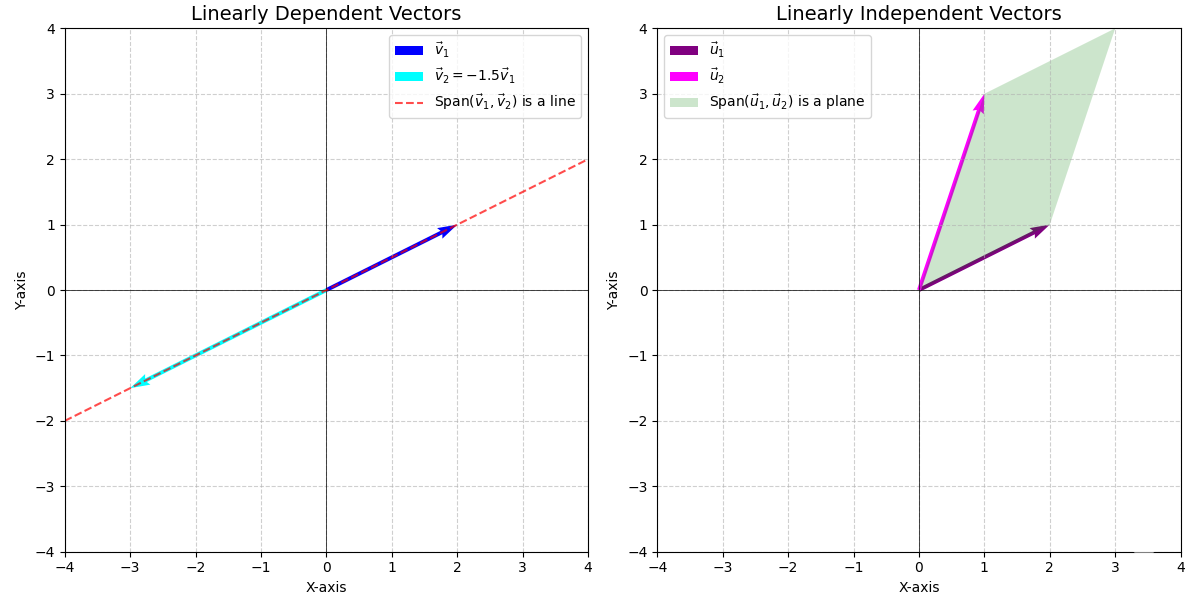
The span of a set of vectors \(\{\vec{v}_1, \dots, \vec{v}_k\}\), denoted \(\text{Span}(\vec{v}_1, \dots, \vec{v}_k)\), is the set of all possible linear combinations of these vectors. Geometrically:
- \(\text{Span}(\vec{v})\) (for \(\vec{v} \neq \vec{0}\)) is the line through the origin containing \(\vec{v}\).
- \(\text{Span}(\vec{v}_1, \vec{v}_2)\) (if \(\vec{v}_1, \vec{v}_2\) are not collinear) is the plane through the origin containing \(\vec{v}_1\) and \(\vec{v}_2\).
- \(\text{Span}(\vec{v}_1, \cdot, \vec{v}_n)\) is the \(n\)-dimensional hyperplane (higher-dimensional analog of lines and planes, “flat” spaces) the origin containing \(\vec{v}_1, \dots, \vec{v}_n\).
 Span and linear combinations in \(\mathbb{R}^2\)
Definition. Linear Independence
A set of vectors \(\{\vec{v}_1, \dots, \vec{v}_k\}\) is linearly independent if the only solution to the equation:
\[c_1\vec{v}_1 + c_2\vec{v}_2 + \dots + c_k\vec{v}_k = \vec{0}\]is \(c_1 = c_2 = \dots = c_k = 0\). If there is any other solution, the set is linearly dependent.
Geometrically, a set of vectors is linearly independent if no vector in the set can be expressed as a linear combination of the others (i.e., no vector lies in the span of the remaining vectors). They each add a new “dimension” to the span.
- Two non-zero vectors are linearly dependent if and only if they are collinear (being scalar multiples of each other, they lie on the same line, which has dimension 1).
- Three vectors in \(\mathbb{R}^3\) are linearly dependent if and only if they are coplanar (lie on the same plane through the origin, which has dimension 2). Thus, for \(k\) vectors, if they are linearly dependent, we have \(\dim \mathrm{Span}(\vec{v}_1, \dots, \vec{v}_k) < k\). Conversely, if \(k\) vectors are linearly independent, they span a \(k\)-dimensional space: \(\dim \mathrm{Span}(\vec{v}_1, \dots, \vec{v}_k) = k\).
Definition. Basis and Dimension
A basis for a vector space (or subspace) \(V\) is a set of vectors \(\mathcal{B} = \{\vec{b}_1, \dots, \vec{b}_n\}\) that satisfies two conditions:
- The vectors in \(\mathcal{B}\) are linearly independent.
- The vectors in \(\mathcal{B}\) span \(V\) (i.e., \(\text{Span}(\vec{b}_1, \dots, \vec{b}_n) = V\)).
The dimension of \(V\), denoted \(\dim(V)\), is the number of vectors in any basis for \(V\).
Geometrically, a basis provides a minimal set of “direction vectors” needed to reach any point in the space. The dimension is the number of such independent directions. For \(\mathbb{R}^n\), the dimension is \(n\). The standard basis for \(\mathbb{R}^n\) consists of vectors \(\vec{e}_1, \dots, \vec{e}_n\), where \(\vec{e}_i\) has a 1 in the \(i\)-th position and 0s elsewhere. For \(\mathbb{R}^2\): \(\vec{e}_1 = \begin{pmatrix} 1 \\ 0 \end{pmatrix}, \vec{e}_2 = \begin{pmatrix} 0 \\ 1 \end{pmatrix}\). For \(\mathbb{R}^3\): \(\vec{e}_1 = \begin{pmatrix} 1 \\ 0 \\ 0 \end{pmatrix}, \vec{e}_2 = \begin{pmatrix} 0 \\ 1 \\ 0 \end{pmatrix}, \vec{e}_3 = \begin{pmatrix} 0 \\ 0 \\ 1 \end{pmatrix}\).
Example. Span and Linear Independence in \(\mathbb{R}^2\)
Let \(\vec{v}_1 = \begin{pmatrix} 1 \\ 1 \end{pmatrix}\) and \(\vec{v}_2 = \begin{pmatrix} -1 \\ 2 \end{pmatrix}\).
Span: \(\text{Span}(\vec{v}_1, \vec{v}_2)\). Can we reach any vector \(\begin{pmatrix} x \\ y \end{pmatrix}\) in \(\mathbb{R}^2\)? We need to find scalars \(c_1, c_2\) such that:
\[c_1 \begin{pmatrix} 1 \\ 1 \end{pmatrix} + c_2 \begin{pmatrix} -1 \\ 2 \end{pmatrix} = \begin{pmatrix} x \\ y \end{pmatrix}\]This gives the system:
\[\begin{cases} c_1 - c_2 = x \\ c_1 + 2c_2 = y \end{cases}\]Subtracting the first from the second: \(3c_2 = y-x \implies c_2 = (y-x)/3\). Substituting back: \(c_1 = x + c_2 = x + (y-x)/3 = (3x+y-x)/3 = (2x+y)/3\). Since we can find \(c_1, c_2\) for any \(x,y\), these vectors span \(\mathbb{R}^2\).
Linear Independence: Are \(\vec{v}_1, \vec{v}_2\) linearly independent? We check if \(c_1\vec{v}_1 + c_2\vec{v}_2 = \vec{0}\) has only the trivial solution \(c_1=c_2=0\).
\[c_1 \begin{pmatrix} 1 \\ 1 \end{pmatrix} + c_2 \begin{pmatrix} -1 \\ 2 \end{pmatrix} = \begin{pmatrix} 0 \\ 0 \end{pmatrix}\]This is the same system as above with \(x=0, y=0\). So, \(c_2 = (0-0)/3 = 0\) and \(c_1 = (2(0)+0)/3 = 0\). Yes, they are linearly independent.
Since \(\{\vec{v}_1, \vec{v}_2\}\) are linearly independent and span \(\mathbb{R}^2\), they form a basis for \(\mathbb{R}^2\). Geometrically, \(\vec{v}_1\) and \(\vec{v}_2\) point in different directions, so together they can “reach” any point on the plane.
Span, Basis & Dimension Exercises:
- Determine if \(\vec{w} = \begin{pmatrix} 7 \\ 0 \end{pmatrix}\) is in the span of \(\vec{v}_1 = \begin{pmatrix} 1 \\ 2 \end{pmatrix}\) and \(\vec{v}_2 = \begin{pmatrix} 3 \\ -1 \end{pmatrix}\).
- Are the vectors \(\begin{pmatrix} 1 \\ 0 \\ 1 \end{pmatrix}, \begin{pmatrix} 0 \\ 1 \\ 1 \end{pmatrix}, \begin{pmatrix} 1 \\ 1 \\ 0 \end{pmatrix}\) linearly independent in \(\mathbb{R}^3\)? Do they form a basis for \(\mathbb{R}^3\)?
- Describe the span of \(\vec{u} = \begin{pmatrix} 1 \\ -1 \\ 2 \end{pmatrix}\) and \(\vec{v} = \begin{pmatrix} -2 \\ 2 \\ -4 \end{pmatrix}\) in \(\mathbb{R}^3\). What is the geometric shape?
- Can a set of two vectors be a basis for \(\mathbb{R}^3\)? Why or why not?
- Can a set of four vectors in \(\mathbb{R}^3\) be linearly independent? Why or why not?
See (Gregory Gunderson, 2021) for more.
3. The Action: Linear Transformations
A transformation \(T: \mathbb{R}^n \to \mathbb{R}^m\) is a function that maps input vectors from \(\mathbb{R}^n\) to output vectors in \(\mathbb{R}^m\). Linear algebra focuses on a special class: linear transformations.
Definition (Geometric). Linear Transformation
A transformation \(T\) is linear if it satisfies two geometric conditions:
- The origin maps to the origin: \(T(\vec{0}) = \vec{0}\).
- Grid lines remain parallel and evenly spaced. Lines remain lines. This means the transformation might stretch, rotate, shear, or reflect the space, but it does so uniformly.
While this geometric picture is highly intuitive, especially in 2D and 3D, relying solely on it can be limiting. To rigorously prove properties of these transformations and to extend these ideas to settings beyond visualizable Euclidean space (like spaces of functions or higher-dimensional data), we need a more formal, algebraic definition. The key is to capture the essence of “preserving grid lines and even spacing” in algebraic terms. This leads us to identify properties like additivity and homogeneity as fundamental. These algebraic properties are not only easier to work with for proving general theorems but also form the basis for generalizing the concept of linearity to other mathematical structures.
This geometric intuition leads to precise algebraic properties:
Derivation. Algebraic Properties from Geometric Intuition
Preservation of Addition (Additivity): Consider vectors \(\vec{u}, \vec{v}\). Their sum \(\vec{u}+\vec{v}\) forms the diagonal of a parallelogram with sides \(\vec{u}\) and \(\vec{v}\). If grid lines and parallelism are preserved, the transformed vectors \(T(\vec{u})\) and \(T(\vec{v})\) must also form a parallelogram, and its diagonal must be \(T(\vec{u}+\vec{v})\). By the parallelogram rule applied to the transformed vectors, this diagonal is also \(T(\vec{u}) + T(\vec{v})\). Thus, for the grid structure to be preserved:
\[T(\vec{u} + \vec{v}) = T(\vec{u}) + T(\vec{v})\]Preservation of Scalar Multiplication (Homogeneity): Consider the vector \(c\vec{v}\). This is \(\vec{v}\) scaled by \(c\). If grid lines remain evenly spaced, scaling before transforming must give the same result as transforming then scaling by the same factor \(c\):
\[T(c\vec{v}) = cT(\vec{v})\]
These two conditions are usually combined into a single, standard algebraic definition:
Theorem. Algebraic Definition of Linear Transformations
A transformation \(T: V \to W\) (where \(V, W\) are vector spaces) is linear if and only if for all vectors \(\vec{x}, \vec{y}\) in \(V\) and all scalars \(a, b\):
\[T(a\vec{x} + b\vec{y}) = aT(\vec{x}) + bT(\vec{y})\]This can be broken down into two simpler conditions:
- \(T(\vec{x} + \vec{y}) = T(\vec{x}) + T(\vec{y})\) (Additivity)
- \(T(c\vec{x}) = cT(\vec{x})\) (Homogeneity)
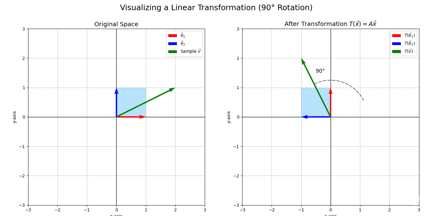
Example. A Rotation Transformation
Let \(T: \mathbb{R}^2 \to \mathbb{R}^2\) be a transformation that rotates every vector counter-clockwise by \(90^\circ\) around the origin.
- Geometrically, this transformation keeps the origin fixed. If you imagine the grid lines, they are rotated, but they remain parallel and evenly spaced (they just form a new, rotated grid). So, it seems linear.
- Let’s check algebraically. A vector \(\vec{v} = \begin{pmatrix} x \\ y \end{pmatrix}\) is rotated to \(T(\vec{v}) = \begin{pmatrix} -y \\ x \end{pmatrix}\).
Additivity: Let \(\vec{u} = \begin{pmatrix} u_1 \\ u_2 \end{pmatrix}\) and \(\vec{v} = \begin{pmatrix} v_1 \\ v_2 \end{pmatrix}\).
\[T(\vec{u}+\vec{v}) = T \begin{pmatrix} u_1+v_1 \\ u_2+v_2 \end{pmatrix} = \begin{pmatrix} -(u_2+v_2) \\ u_1+v_1 \end{pmatrix} = \begin{pmatrix} -u_2-v_2 \\ u_1+v_1 \end{pmatrix}\] \[T(\vec{u}) + T(\vec{v}) = \begin{pmatrix} -u_2 \\ u_1 \end{pmatrix} + \begin{pmatrix} -v_2 \\ v_1 \end{pmatrix} = \begin{pmatrix} -u_2-v_2 \\ u_1+v_1 \end{pmatrix}\]They are equal.
Homogeneity: Let \(c\) be a scalar.
\[T(c\vec{v}) = T \begin{pmatrix} cx \\ cy \end{pmatrix} = \begin{pmatrix} -cy \\ cx \end{pmatrix}\] \[cT(\vec{v}) = c \begin{pmatrix} -y \\ x \end{pmatrix} = \begin{pmatrix} -cy \\ cx \end{pmatrix}\]They are equal. Since both conditions hold, the rotation is a linear transformation.
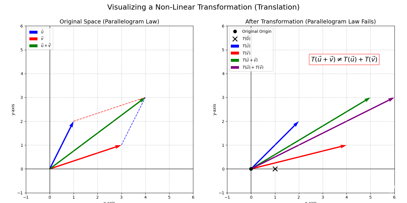
Example. A Non-Linear Transformation
Consider \(T: \mathbb{R}^2 \to \mathbb{R}^2\) defined by \(T\begin{pmatrix} x \\ y \end{pmatrix} = \begin{pmatrix} x+1 \\ y \end{pmatrix}\). This is a translation (shift).
Let’s check \(T(\vec{0})\): \(T\begin{pmatrix} 0 \\ 0 \end{pmatrix} = \begin{pmatrix} 0+1 \\ 0 \end{pmatrix} = \begin{pmatrix} 1 \\ 0 \end{pmatrix} \neq \vec{0}\).
Since the origin is not fixed (or by failing homogeneity/additivity), this transformation is not linear.
Linear Transformation Exercises:
- Is \(T\begin{pmatrix} x \\ y \end{pmatrix} = \begin{pmatrix} x^2 \\ y \end{pmatrix}\) a linear transformation? Justify.
- Is \(T\begin{pmatrix} x \\ y \\ z \end{pmatrix} = \begin{pmatrix} x-y \\ y-z \\ z-x \end{pmatrix}\) a linear transformation? Justify.
- Describe geometrically the transformation \(T\begin{pmatrix} x \\ y \end{pmatrix} = \begin{pmatrix} x \\ 0 \end{pmatrix}\). Is it linear? This is a projection onto the x-axis.
- If \(T\) is a linear transformation, prove that \(T(\vec{0}) = \vec{0}\). (Hint: Use \(T(c\vec{x})=cT(\vec{x})\) with \(c=0\)).
- Suppose \(T: \mathbb{R}^2 \to \mathbb{R}^2\) is a linear transformation such that \(T\begin{pmatrix} 1 \\ 0 \end{pmatrix} = \begin{pmatrix} 2 \\ 3 \end{pmatrix}\) and \(T\begin{pmatrix} 0 \\ 1 \end{pmatrix} = \begin{pmatrix} -1 \\ 1 \end{pmatrix}\). Find \(T\begin{pmatrix} 5 \\ 7 \end{pmatrix}\).
4. Encoding Linear Transformations: The Matrix
A key insight is that any linear transformation \(T: \mathbb{R}^n \to \mathbb{R}^m\) is completely determined by its action on the standard basis vectors of \(\mathbb{R}^n\).
Derivation. Matrix of a Linear Transformation
Let \(\{\vec{e}_1, \dots, \vec{e}_n\}\) be the standard basis for \(\mathbb{R}^n\).
Any vector \(\vec{x} \in \mathbb{R}^n\) can be written as \(\vec{x} = x_1\vec{e}_1 + x_2\vec{e}_2 + \dots + x_n\vec{e}_n\).
Applying a linear transformation \(T\):
\[\begin{aligned} T(\vec{x}) &= T(x_1\vec{e}_1 + x_2\vec{e}_2 + \dots + x_n\vec{e}_n) \\ &= T(x_1\vec{e}_1) + T(x_2\vec{e}_2) + \dots + T(x_n\vec{e}_n) && \text{(by additivity)} \\ &= x_1 T(\vec{e}_1) + x_2 T(\vec{e}_2) + \dots + x_n T(\vec{e}_n) && \text{(by homogeneity)} \end{aligned}\]This shows that \(T(\vec{x})\) is a linear combination of the vectors \(T(\vec{e}_1), T(\vec{e}_2), \dots, T(\vec{e}_n)\). These transformed basis vectors are vectors in \(\mathbb{R}^m\). Let’s define a matrix \(A\) whose columns are precisely these transformed basis vectors:
\[A = \begin{pmatrix} \vert & \vert & & \vert \\ T(\vec{e}_1) & T(\vec{e}_2) & \dots & T(\vec{e}_n) \\ \vert & \vert & & \vert \end{pmatrix}\]Then the expression \(x_1 T(\vec{e}_1) + x_2 T(\vec{e}_2) + \dots + x_n T(\vec{e}_n)\) is exactly the definition of the matrix-vector product \(A\vec{x}\), where \(\vec{x} = \begin{pmatrix} x_1 \\ \vdots \\ x_n \end{pmatrix}\). So, \(T(\vec{x}) = A\vec{x}\).
Theorem. Matrix Representation of Linear Transformations
For any linear transformation \(T: \mathbb{R}^n \to \mathbb{R}^m\), there exists a unique \(m \times n\) matrix \(A\) such that \(T(\vec{x}) = A\vec{x}\) for all \(\vec{x}\) in \(\mathbb{R}^n\). The columns of this matrix \(A\) are the images of the standard basis vectors under \(T\): \(A = \begin{pmatrix} T(\vec{e}_1) & T(\vec{e}_2) & \dots & T(\vec{e}_n) \end{pmatrix}\).
Conversely, any transformation defined by \(T(\vec{x}) = A\vec{x}\) for some matrix \(A\) is a linear transformation.
This establishes a fundamental link: matrices are linear transformations (in finite Euclidean spaces relative to standard bases).
Example. Matrix for \(90^\circ\) Rotation
Consider the \(90^\circ\) counter-clockwise rotation \(T: \mathbb{R}^2 \to \mathbb{R}^2\).
The standard basis vectors are \(\vec{e}_1 = \begin{pmatrix} 1 \\ 0 \end{pmatrix}\) and \(\vec{e}_2 = \begin{pmatrix} 0 \\ 1 \end{pmatrix}\).
- \(T(\vec{e}_1) = T\begin{pmatrix} 1 \\ 0 \end{pmatrix} = \begin{pmatrix} 0 \\ 1 \end{pmatrix}\) (rotating \((1,0)\) by \(90^\circ\) CCW lands on \((0,1)\)).
- \(T(\vec{e}_2) = T\begin{pmatrix} 0 \\ 1 \end{pmatrix} = \begin{pmatrix} -1 \\ 0 \end{pmatrix}\) (rotating \((0,1)\) by \(90^\circ\) CCW lands on \((-1,0)\)).
The matrix \(A\) has these as columns:
\[A = \begin{pmatrix} 0 & -1 \\ 1 & 0 \end{pmatrix}\]So, for any vector \(\vec{x} = \begin{pmatrix} x \\ y \end{pmatrix}\), \(T(\vec{x}) = A\vec{x} = \begin{pmatrix} 0 & -1 \\ 1 & 0 \end{pmatrix} \begin{pmatrix} x \\ y \end{pmatrix} = \begin{pmatrix} -y \\ x \end{pmatrix}\), which matches our earlier formula.
Tip. Indexing Notation for Matrix Entries
Since we can encode a matrix’s entries in a rectangular table, we can iterate over two indices to identify any entry. So we write \(A=A_{ij}\), where the first index \(i\) loops over the horizontal rows and the second index \(j\) loops over the vertical columns.
Example. Indexing Notation for Matrix Entries
For \(A\in \mathbb{R}^{3 \times 2}\), i.e. 3 rows and 2 columns:
\[A = \begin{pmatrix} A_{11} & A_{12} \\ A_{21} & A_{22} \\ A_{31} & A_{32} \end{pmatrix}\]and the matrix is determined by its entries.
Exercise. Identity Matrix
Think about a square matrix \(I\in \mathbb{R}^{n \times n}\) where \(I_{ij}=1\) if \(i=j\) or \(0\) otherwise. \(I\) is called the identity matrix. Basically, everything along the main diagonal (from top left to bottom right) is \(1\), and everything else is \(0\).
\[I = \begin{pmatrix} 1 & 0 & 0 & \cdots & 0 \\ 0 & 1 & 0 & \cdots & 0 \\ 0 & 0 & 1 & \cdots & 0 \\ \vdots& & & \ddots & \\ 0 & 0 & 0 & \cdots & 1 \end{pmatrix}\]What is the effect of the linear transformation \(I\)? Hint: look at the form of our basis vectors \(e_i\) again.
4.1. Composition of Transformations and Matrix Multiplication
If you apply one linear transformation \(T_1\) (matrix \(A_1\)) and then another \(T_2\) (matrix \(A_2\)), the combined effect is also a linear transformation \(T = T_2 \circ T_1\) (apply \(T_1\) first, then \(T_2\)). Its matrix is the product \(A = A_2 A_1\). Geometrically, matrix multiplication corresponds to composing the geometric actions. The order matters!
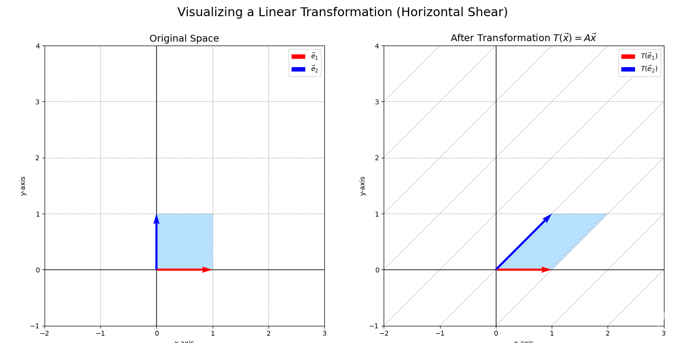
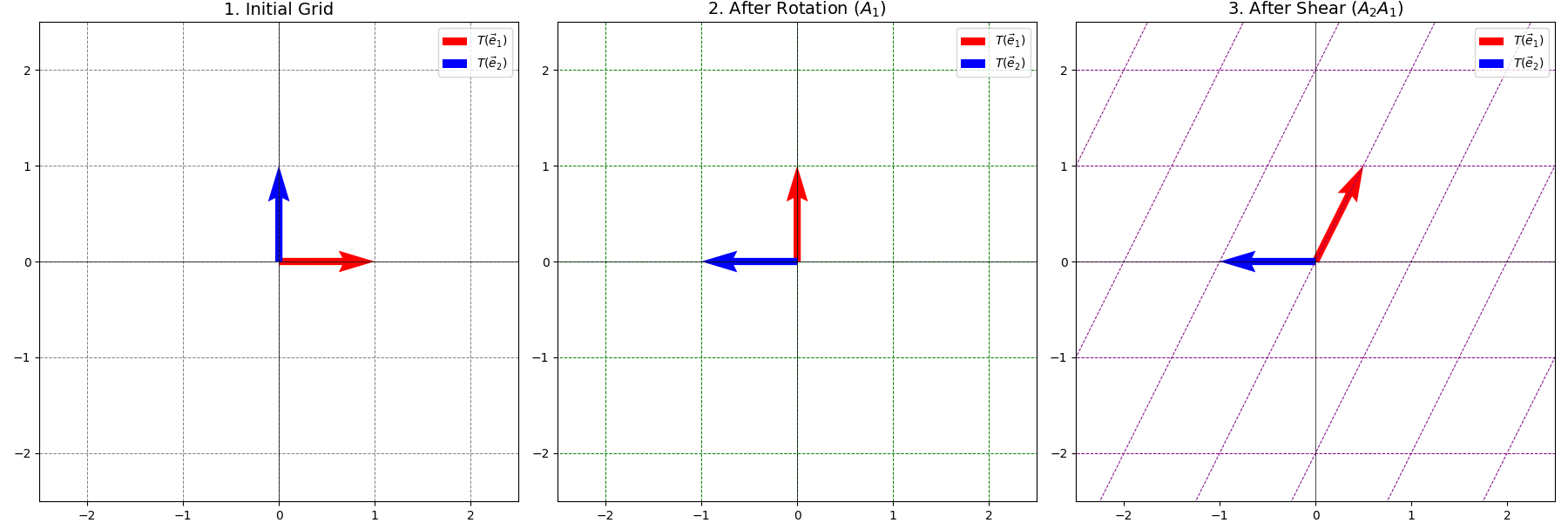
Example. Composition: Rotate then Shear
Let \(T_1\) be a rotation by \(90^\circ\) counter-clockwise: \(A_1 = \begin{pmatrix} 0 & -1 \\ 1 & 0 \end{pmatrix}\). Let \(T_2\) be a horizontal shear that maps \(\vec{e}_2\) to \(\begin{pmatrix} 0.5 \\ 1 \end{pmatrix}\) and leaves \(\vec{e}_1\) fixed: \(A_2 = \begin{pmatrix} 1 & 0.5 \\ 0 & 1 \end{pmatrix}\). The transformation “rotate then shear” (\(T_2 \circ T_1\)) has matrix \(A = A_2 A_1\):
\[A = \begin{pmatrix} 1 & 0.5 \\ 0 & 1 \end{pmatrix} \begin{pmatrix} 0 & -1 \\ 1 & 0 \end{pmatrix} = \begin{pmatrix} (1)(0)+(0.5)(1) & (1)(-1)+(0.5)(0) \\ (0)(0)+(1)(1) & (0)(-1)+(1)(0) \end{pmatrix} = \begin{pmatrix} 0.5 & -1 \\ 1 & 0 \end{pmatrix}\]Let’s see where \(\vec{e}_1\) goes under the composite transformation:
\[T_1(\vec{e}_1) = \begin{pmatrix} 0 \\ 1 \end{pmatrix} = \vec{e}_2\] \[T_2(\vec{e}_2) = \begin{pmatrix} 0.5 \\ 1 \end{pmatrix}\]This is the first column of \(A\). Correct.
Let’s see where \(\vec{e}_2\) goes:
\[T_1(\vec{e}_2) = \begin{pmatrix} -1 \\ 0 \end{pmatrix} = -\vec{e}_1\] \[T_2(-\vec{e}_1) = \begin{pmatrix} 1 & 0.5 \\ 0 & 1 \end{pmatrix} \begin{pmatrix} -1 \\ 0 \end{pmatrix} = \begin{pmatrix} -1 \\ 0 \end{pmatrix}\]This is the second column of \(A\). Correct.
Matrix & Transformation Exercises:
- Find the matrix for the linear transformation \(T: \mathbb{R}^2 \to \mathbb{R}^2\) that reflects vectors across the x-axis.
- Find the matrix for the linear transformation \(T: \mathbb{R}^2 \to \mathbb{R}^2\) that projects vectors onto the line \(y=x\). (Hint: Where do \(\vec{e}_1\) and \(\vec{e}_2\) land?)
- Find the matrix for the linear transformation \(T: \mathbb{R}^3 \to \mathbb{R}^2\) defined by \(T\begin{pmatrix} x \\ y \\ z \end{pmatrix} = \begin{pmatrix} x+y \\ y-z \end{pmatrix}\).
- If \(A = \begin{pmatrix} 1 & 0 \\ 0 & 0 \end{pmatrix}\), describe geometrically what the transformation \(T(\vec{x}) = A\vec{x}\) does to vectors in \(\mathbb{R}^2\).
- If \(T: \mathbb{R}^n \to \mathbb{R}^m\) and \(S: \mathbb{R}^m \to \mathbb{R}^p\) are linear transformations with matrices \(A\) and \(B\) respectively, the composition \(S \circ T\) (meaning \(S(T(\vec{x}))\)) is also a linear transformation. What is its matrix? (Hint: Consider the action of the composition on the basis vectors \(e_i\in \mathbb{R}^n\). Use matrix indexing notation for easier calculations.)
See (Gregory Gunderson, 2022) and (Gregory Gunderson, 2018) for more.
5. Measuring Geometric Change: Determinants
For square matrices \(A\) (representing \(T: \mathbb{R}^n \to \mathbb{R}^n\)), the determinant measures how the transformation scales volume and affects orientation.
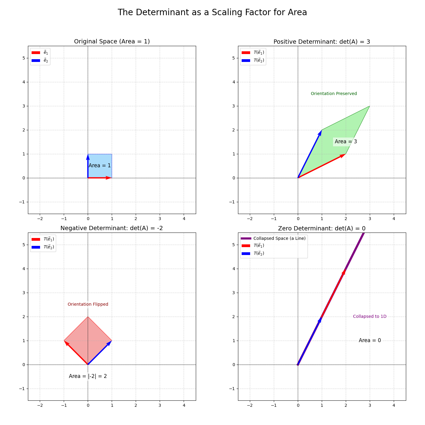
Definition (Geometric). Determinant
The determinant of an \(n \times n\) matrix \(A\), denoted \(\det(A)\) or \(\vert A \vert\), is the signed volume of the parallelepiped formed by the images of the standard basis vectors (thus the unit hypercube \([0,1]^n\)) under the transformation \(T(\vec{x}) = A\vec{x}\). (These images are the columns of \(A\)). The “volume” refers to area in \(\mathbb{R}^2\), volume in \(\mathbb{R}^3\), and hypervolume in \(\mathbb{R}^n\).
- \(\vert \det(A) \vert\): The factor by which \(T\) scales any volume/area.
- Sign of \(\det(A)\):
- \(\det(A) > 0\): Preserves orientation. (e.g. a rotation)
- \(\det(A) < 0\): Reverses orientation (e.g. a reflection).
- \(\det(A) = 0\): Collapses space to a lower dimension. This means the columns of \(A\) are linearly dependent, and the matrix \(A\) is singular (not invertible). The “volume” of the transformed parallelepiped is zero because it’s flattened into a lower-dimensional shape (a line or a point if in 2D, a plane or line or point if in 3D, etc.).
Theorem. Algebraic Definition of Determinant
The determinant can be defined algebraically through properties:
\[\det(A) = a(ei - fh) - b(di - fg) + c(dh - eg)\]
- \(\det(I) = 1\) (Identity matrix preserves volume and orientation).
- Multilinearity: If a row (or column) is multiplied by a scalar \(c\), the determinant is multiplied by \(c\). If a row is a sum of two vectors, the determinant is the sum of determinants using each vector.
- Alternating: Swapping two rows (or columns) multiplies the determinant by \(-1\). These lead to computational formulas. For \(A = \begin{pmatrix} a & b \\ c & d \end{pmatrix}\), \(\det(A) = ad - bc\). For \(A = \begin{pmatrix} a & b & c \\ d & e & f \\ g & h & i \end{pmatrix}\),
For larger matrices, cofactor expansion or row reduction methods are used.
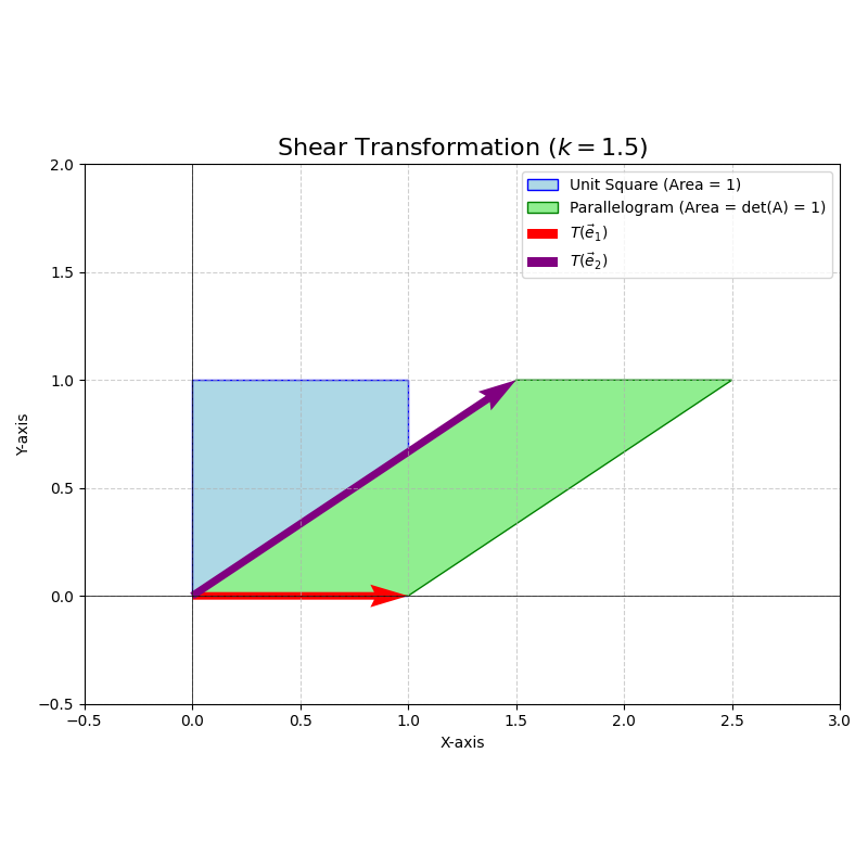
Example. Determinant of a Shear Transformation
Consider the shear matrix \(A = \begin{pmatrix} 1 & k \\ 0 & 1 \end{pmatrix}\) in \(\mathbb{R}^2\).
\[\det(A) = (1)(1) - (k)(0) = 1\]Geometrically, a shear transformation maps a square to a parallelogram with the same base and height. Thus, the area is preserved. \(\vert \det(A) \vert = 1\) confirms this. Since \(\det(A) = 1 > 0\), orientation is also preserved. The standard basis vector \(\vec{e}_1 = \begin{pmatrix} 1 \\ 0 \end{pmatrix}\) maps to \(\begin{pmatrix} 1 \\ 0 \end{pmatrix}\). The standard basis vector \(\vec{e}_2 = \begin{pmatrix} 0 \\ 1 \end{pmatrix}\) maps to \(\begin{pmatrix} k \\ 1 \end{pmatrix}\). The unit square (formed by \(\vec{e}_1, \vec{e}_2\)) is transformed into a parallelogram with vertices at \((0,0), (1,0), (k,1), (1+k,1)\). The area of this parallelogram is base \(\times\) height \(= 1 \times 1 = 1\).
Important Properties of Determinants:
- \(\det(AB) = \det(A)\det(B)\). (The scaling factor of a composite transformation is the product of individual scaling factors).
- \(\det(A^T) = \det(A)\).
- \(A\) is invertible if and only if \(\det(A) \neq 0\).
- If \(A\) is invertible, \(\det(A^{-1}) = 1/\det(A)\).
Determinant Exercises:
- Calculate the determinant of \(A = \begin{pmatrix} 3 & 1 \\ -2 & 4 \end{pmatrix}\). What does this tell you about the area scaling and orientation?
- If \(A = \begin{pmatrix} 2 & 0 & 0 \\ 0 & 3 & 0 \\ 0 & 0 & -1 \end{pmatrix}\), what is \(\det(A)\)? Interpret geometrically.
- Show that if a matrix has a row or column of zeros, its determinant is 0.
- If \(A\) is an \(n \times n\) matrix and \(c\) is a scalar, what is \(\det(cA)\) in terms of \(\det(A)\) and \(n\)?
- Without calculating, explain why \(\det \begin{pmatrix} 1 & 2 & 3 \\ 1 & 2 & 3 \\ 4 & 5 & 6 \end{pmatrix} = 0\).
6. Solving Problems: Systems of Linear Equations
A system of linear equations can be written in matrix form as \(A\vec{x} = \vec{b}\). Having explored transformations and determinants, we can interpret this geometrically.
Interpretation. \(A\vec{x} = \vec{b}\)
- Transformation View: We are looking for a vector \(\vec{x}\) in the input space that the transformation \(A\) maps to the vector \(\vec{b}\) in the output space.
- If \(\det(A) \neq 0\) (for square \(A\)), \(A\) is invertible. The transformation maps \(\mathbb{R}^n\) to \(\mathbb{R}^n\) without loss of dimension. A unique \(\vec{x} = A^{-1}\vec{b}\) exists. Geometrically, \(A^{-1}\) “undoes” the transformation of \(A\).
- If \(\det(A) = 0\) (for square \(A\)) or if \(A\) is not square, the transformation might collapse space. A solution exists if and only if \(\vec{b}\) is in the column space of \(A\) (the span of the columns of \(A\), i.e., the image of the transformation). The concept of column space and its relation to solutions will be explored more in Part 2 (Section 10, The Transpose). If a solution exists, it might not be unique.
- Linear Combination View: Let the columns of \(A\) be \(\vec{a}_1, \dots, \vec{a}_n\). Then \(A\vec{x} = x_1\vec{a}_1 + \dots + x_n\vec{a}_n\). So, \(A\vec{x} = \vec{b}\) asks: “Is \(\vec{b}\) a linear combination of the columns of \(A\)? If so, what are the coefficients \(x_1, \dots, x_n\)?” In other words, is \(\vec{b}\) in the column space of \(A\)?
- Geometric Intersection View (for \(\mathbb{R}^2, \mathbb{R}^3\)): Each equation in the system represents a line (in \(\mathbb{R}^2\)) or a plane (in \(\mathbb{R}^3\)). Solving the system means finding the point(s) of intersection of these geometric objects.
- Unique solution: Lines/planes intersect at a single point. (Corresponds to \(\det(A) \neq 0\) for \(n \times n\) systems).
- No solution: Lines are parallel / planes don’t intersect at a common point. (\(\vec{b}\) is not in Col(A)).
- Infinitely many solutions: Lines are identical / planes intersect along a line or are identical. (\(\vec{b}\) is in Col(A), and the null space of A is non-trivial, meaning there are free variables. The null space will be discussed in Part 2).
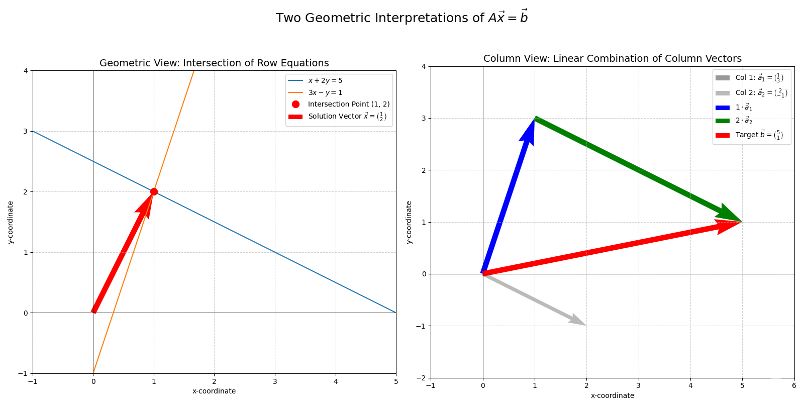
Example. System of Equations
Consider the system:
\[\begin{cases} x + 2y = 5 \\ 3x - y = 1 \end{cases}\]In matrix form: \(\begin{pmatrix} 1 & 2 \\ 3 & -1 \end{pmatrix} \begin{pmatrix} x \\ y \end{pmatrix} = \begin{pmatrix} 5 \\ 1 \end{pmatrix}\). Let \(A = \begin{pmatrix} 1 & 2 \\ 3 & -1 \end{pmatrix}\), \(\vec{x} = \begin{pmatrix} x \\ y \end{pmatrix}\), \(\vec{b} = \begin{pmatrix} 5 \\ 1 \end{pmatrix}\). Here, \(\det(A) = (1)(-1) - (2)(3) = -1 - 6 = -7 \neq 0\). So, A is invertible and a unique solution exists. The transformation \(A\) maps the plane to itself without collapsing it. We are looking for the unique vector \(\vec{x}\) that gets mapped to \(\vec{b}\). (Solving this system yields \(x=1, y=2\). So \(\vec{x}=\begin{pmatrix} 1 \\ 2 \end{pmatrix}\) is the solution.)
System of Equations Exercises:
- Write the system \(2x-y=3, x+3y=-2\) in the form \(A\vec{x}=\vec{b}\). Calculate \(\det(A)\). Does a unique solution exist?
- Consider \(A = \begin{pmatrix} 1 & -1 \\ -2 & 2 \end{pmatrix}\). Can you find an \(\vec{x}\) such that \(A\vec{x} = \begin{pmatrix} 3 \\ 0 \end{pmatrix}\)? What about \(A\vec{x} = \begin{pmatrix} 1 \\ -2 \end{pmatrix}\)? Interpret geometrically (hint: what does \(A\) do to vectors? Are its columns linearly independent? What is \(\det(A)\)?).
- If \(A\vec{x}=\vec{b}\) has a unique solution for a square matrix \(A\), what does this imply about the columns of \(A\)? What does it imply about the transformation \(T(\vec{x})=A\vec{x}\)? What is \(\det(A)\)?
- Describe the solution set of \(A\vec{x}=\vec{0}\) (the homogeneous system). What is the geometric meaning of this set (the null space of \(A\))? (The null space will be discussed more formally in Part 2).
- If \(\vec{p}\) is a particular solution to \(A\vec{x}=\vec{b}\), and \(\vec{h}\) is any solution to \(A\vec{x}=\vec{0}\), show that \(\vec{p}+\vec{h}\) is also a solution to \(A\vec{x}=\vec{b}\). Geometrically, this means the solution set to \(A\vec{x}=\vec{b}\) is a translation of the null space.
7. The Power of Linearity: From Local Definition to Global Property
A profound consequence of linearity is that the behavior of a linear transformation or its associated measures, when understood for simple, “local” elements, dictates its “global” behavior across the entire space. This principle makes linear systems remarkably predictable.
Principle. Local Information Defines Global Behavior in Linear Systems
For linear transformations \(T(\vec{x}) = A\vec{x}\), how the transformation acts on a fundamental local structure (like the basis vectors near the origin, or individual solutions to an equation) completely and uniformly determines its behavior across the entire space. Properties derived from this local action become global characteristics.
Let’s explore this with concrete examples covered in this part of the course:
1. The Matrix Itself: Local Action on Basis Vectors Defines Global Transformation
- Local Information: As we saw in Section 4, a linear transformation \(T: \mathbb{R}^n \to \mathbb{R}^m\) is entirely determined by where it sends the standard basis vectors \(\vec{e}_1, \dots, \vec{e}_n\). These are just \(n\) specific vectors. The matrix \(A\) of the transformation simply lists these \(n\) transformed vectors \(T(\vec{e}_i)\) as its columns. This describes what happens to a small set of “test vectors” originating at the origin.
- Global Consequence: Due to linearity (\(T(c_1\vec{v}_1 + \dots + c_k\vec{v}_k) = c_1T(\vec{v}_1) + \dots + c_kT(\vec{v}_k)\)), this “local” knowledge of where the basis vectors land allows us to determine where any vector \(\vec{x}\) in the entire space is transformed. Since any \(\vec{x}\) is a linear combination of basis vectors (\(\vec{x} = x_1\vec{e}_1 + \dots + x_n\vec{e}_n\)), its image is \(A\vec{x} = x_1 T(\vec{e}_1) + \dots + x_n T(\vec{e}_n)\). The transformation rules (stretching, rotating, shearing) encoded in \(A\) by its action on the basis vectors apply uniformly across the entire space, preserving the overall grid structure.
2. The Determinant: Local Volume Change Defines Global Volume Scaling
- Local Information: The geometric definition of \(\det(A)\) (for an \(n \times n\) matrix \(A\)) is the signed volume of the parallelepiped formed by the transformed standard basis vectors \(T(\vec{e}_1), \dots, T(\vec{e}_n)\). This specifically describes how the unit hypercube (a small, local region at the origin) changes in volume and orientation.
- Global Consequence: Because a linear transformation warps space consistently and uniformly everywhere (as detailed in the collapsible block in Section 5 of the full LA course, or by considering infinitesimal regions), this single, locally-derived scaling factor \(\vert\det(A)\vert\) applies to any region in the space, no matter its shape, size, or location. The area (or volume, or hypervolume) of any arbitrarily large or complex shape will be scaled by exactly this same factor. The orientation change (flip or no flip) indicated by the sign of \(\det(A)\) is also a global property.
This “local determines global” characteristic is a cornerstone of why linear algebra is so powerful and predictable. Other examples involving eigenvalues and the structure of solution sets (related to the null space and column space) will be explored in Part 2 of this Linear Algebra series.
The geometric viewpoint of linear algebra is highly useful to reason about some facts that seem intuitively true, but not immediately obvious to prove. (However, beware the “curse of dimensionality”, where certain intuitions in low dimensions may not hold in higher dimensions.)
Here are some examples.
- Similarity in Geometry: In geometry, it is known that scaling a shape by a factor of \(k\) changes its volume by a factor of \(k^n\), where \(n\) is the dimension of the space. This feels somewhat correct, but hard to fully justify intuitively. However, with the properties of the determinant, this is obvious: we are applying a scaling transformation \(kI\) where \(I\) is the identity transformation, i.e. each basis vector is scaled by a factor of \(k\). From the globality of the determinant, the whole shape’s volume is scaled by \(det(kI)=k^n\).
- Cavalier’s principle: Cavalier’s principle states that two regions that differ only up to translations in a single direction have equal volume. In linear algebraic terms, is simply that a shearing transformation does not affect volume.
Here are some concrete examples of intuition it provides.
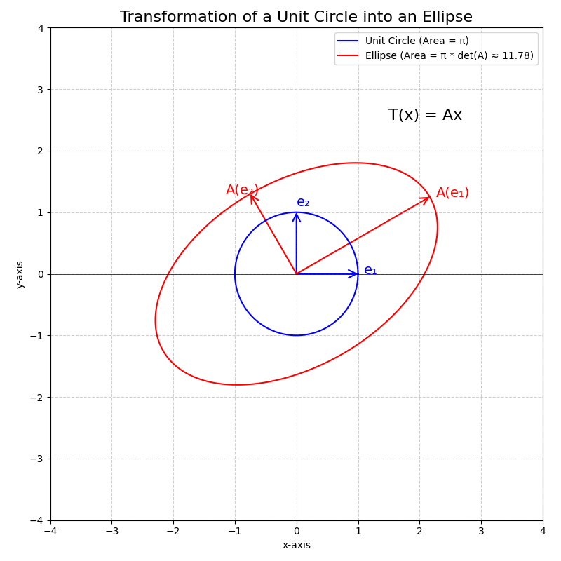
- Area of an ellipse: You might have derived the formula for the area enclosed by an ellipse in multivariable calculus, and you would find this procedure quite tedious. However, knowing that the area of the unit disk is \(\pi\) is sufficient to conclude that, by appropriately rotating the basis vectors and scaling them by the lengths of the semi-diagonals of the ellipse \(a\) and \(b\), the area of the ellipse is \(\pi \cdot a \cdot b\).
Area of a Parallelogram from its Defining Vectors: The definition of the determinant tells us that \(\vert\det(A)\vert\) is the factor by which the transformation \(T(\vec{x})=A\vec{x}\) scales areas (in 2D) or volumes (in 3D). This arises because a linear transformation maps the standard basis vectors, which form a unit square (in 2D) or unit cube (in 3D) of area/volume 1, to a parallelogram or parallelepiped whose area/volume is \(\vert\det(A)\vert\).
We can use this directly: if we want to find the area of a parallelogram spanned by two vectors \(\vec{u}\) and \(\vec{v}\) in \(\mathbb{R}^2\), we can construct a matrix \(M\) whose columns are these vectors: \(M = [\vec{u} \ \vec{v}]\). The linear transformation \(T(\vec{x}) = M\vec{x}\) maps the standard basis vector \(\vec{e}_1 = \begin{pmatrix} 1 \\ 0 \end{pmatrix}\) to \(\vec{u}\) and \(\vec{e}_2 = \begin{pmatrix} 0 \\ 1 \end{pmatrix}\) to \(\vec{v}\). Thus, the unit square spanned by \(\vec{e}_1\) and \(\vec{e}_2\) is transformed into the parallelogram spanned by \(\vec{u}\) and \(\vec{v}\). The area of this parallelogram is therefore \(\vert \det(M) \vert \times \text{Area}(\text{unit square}) = \vert \det(M) \vert \times 1 = \vert \det(M) \vert\).
For example, if \(\vec{u} = \begin{pmatrix} a \\ b \end{pmatrix}\) and \(\vec{v} = \begin{pmatrix} c \\ d \end{pmatrix}\), then \(M = \begin{pmatrix} a & c \\ b & d \end{pmatrix}\), and the area is \(\vert ad - bc \vert\). This provides a fundamental geometric interpretation for the determinant computation: it’s the signed area (or volume) of the shape formed by its column vectors. This is a direct consequence of the local-to-global scaling property, applied to the specific case where the “shape” is defined by the vectors themselves relative to the origin. In \(\mathbb{R}^3\), the volume of the parallelepiped spanned by three vectors \(\vec{u}, \vec{v}, \vec{w}\) is similarly given by \(\vert \det([\vec{u} \ \vec{v} \ \vec{w}]) \vert\).
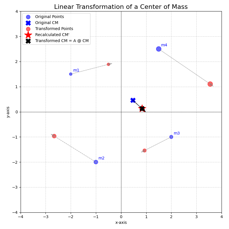
Transformation of the Center of Mass: Consider a system of \(k\) point masses \(m_1, m_2, \dots, m_k\) located at positions \(\vec{p}_1, \vec{p}_2, \dots, \vec{p}_k\) in \(\mathbb{R}^n\). The center of mass of this system is a weighted average of the positions:
\[\vec{R}_{CM} = \frac{m_1\vec{p}_1 + m_2\vec{p}_2 + \dots + m_k\vec{p}_k}{m_1 + m_2 + \dots + m_k} = \frac{\sum_{i=1}^k m_i \vec{p}_i}{M_{total}}\]where \(M_{total} = \sum_{i=1}^k m_i\) is the total mass of the system.
Now, suppose we apply a linear transformation \(T(\vec{x}) = A\vec{x}\) to every point mass in the system, so their new positions become \(\vec{p}_i' = A\vec{p}_i\). What is the new center of mass, \(\vec{R}_{CM}'\)?
\[\vec{R}_{CM}' = \frac{\sum_{i=1}^k m_i \vec{p}_i'}{M_{total}} = \frac{\sum_{i=1}^k m_i (A\vec{p}_i)}{M_{total}}\]Using the properties of linear transformations (specifically, that scalar multiplication commutes with the transformation, \(m_i(A\vec{p}_i) = A(m_i\vec{p}_i)\), and that the transformation distributes over vector addition, \(A(\vec{x}+\vec{y}) = A\vec{x} + A\vec{y}\), which extends to sums), we can factor \(A\) out of the summation:
\[\sum_{i=1}^k m_i (A\vec{p}_i) = \sum_{i=1}^k A (m_i \vec{p}_i) = A \left( \sum_{i=1}^k m_i \vec{p}_i \right)\]Substituting this back into the expression for \(\vec{R}_{CM}'\):
\[\vec{R}_{CM}' = \frac{A \left(\sum_{i=1}^k m_i \vec{p}_i\right)}{M_{total}} = A \left( \frac{\sum_{i=1}^k m_i \vec{p}_i}{M_{total}} \right)\]This elegantly simplifies to:
\[\vec{R}_{CM}' = A \vec{R}_{CM}\]This result demonstrates that the center of mass of the transformed system is simply the transformation of the original center of mass. Instead of recomputing the center of mass from all \(k\) new positions (a potentially tedious “local” recalculation), we can apply the linear transformation \(A\) just once to the original, “global” center of mass vector \(\vec{R}_{CM}\). This powerful simplification is a direct consequence of linearity, showing how the transformation’s consistent action on individual components translates to a consistent action on an aggregate property derived from them.
Conclusion for Part 1
This first part of our linear algebra crash course has laid the groundwork by introducing vectors, vector spaces, the fundamental operations, and the crucial concept of linear transformations and their matrix representations. We’ve seen how matrices encode geometric actions like rotations, shears, and scalings, and how determinants quantify the change in volume and orientation caused by these transformations. We also touched upon how these ideas connect to solving systems of linear equations.
Understanding these foundational concepts is essential before moving on to more advanced topics. Part 2 will build upon this base to explore orthogonality, projections, change of basis, eigenvalues and eigenvectors, special types of matrices, powerful matrix decompositions like SVD, and the abstract notion of vector spaces. These further topics will reveal deeper structural properties of linear transformations and provide tools critical for many applications, including machine learning.
Make sure you’re comfortable with the material here before proceeding to Part 2.
Further Reading
- Grant Sanderson. (2025). Essence of Linear Algebra - YouTube. https://www.youtube.com/playlist?list=PLZHQObOWTQDPD3MizzM2xVFitgF8hE_ab
- Gregory Gunderson. (2018). A Geometrical Understanding of Matrices. https://gregorygundersen.com/blog/2018/10/24/matrices/
- Gregory Gunderson. (2021). Linear Independence, Basis, and the Gram–Schmidt Algorithm. https://gregorygundersen.com/blog/2021/04/24/linear-independence/
- Gregory Gunderson. (2022). Matrices as Functions, Matrices as Data. https://gregorygundersen.com/blog/2022/08/28/matrices-as-functions-and-data/
- Gregory Gunderson. (2018). Two Forms of the Dot Product. https://gregorygundersen.com/blog/2018/06/26/dot-product/
- James Maynard. (2020). Linear Algebra II: Oxford Mathematics 1st Year Student Lecture - James Maynard - YouTube. https://www.youtube.com/watch?v=pQhVDRojC1U